In this very first tutorial we will describe how to solve initial value problems using Houdini. We will first play this through for an first order ODE – the Lorenz system – before you apply the solver to compute the trajectories of charged particles in a static magnetic field.
Consider a smooth vector field \(f\colon \mathbb R^n\to \mathbb R^n\). We are interested in the solutions \(y\colon \mathbb R \to \mathbb R^n\) of the equation \(y^\prime(t) = f(y(t))\) with \(y(t_0) = y_0\in \mathbb R^n\).
The most naive way to numerically approximate a solution is to successively perform linear steps along the tangent. This leads to the so called Euler method: For a given small time step \(h>0\), we put \[y_{k+1} = y_k + h\,f(y_k).\]
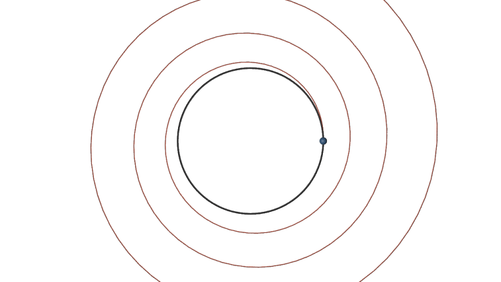
Certainly, we cannot expect high accuracy. E.g., if \(f\colon \mathbb C \to \mathbb C\) is given by \(f(z) = iz\), the exact solutions are circles, while the outcome of the Euler method drifts away from the circle and forms a discrete spiral.
The Euler method is easily implemented using Houdini’s Solver node. Here is how such a network may look like (inside a geometry node):

The Attribute Wrangle node “init trajectory” just takes the initial point (center of a sphere primitive) and turns it in an open polygon (polyline):
|
1 2 3 4 5 |
// add for initial point (Input1) // a curve (polyline) to the curr node geometry vector y0 = point(1,"P",0); int curve = addprim(0,"polyline"); addvertex(0,curve,addpoint(0,y0)); |
The Euler step is performed inside a solver node. Let us dive into the solver node:
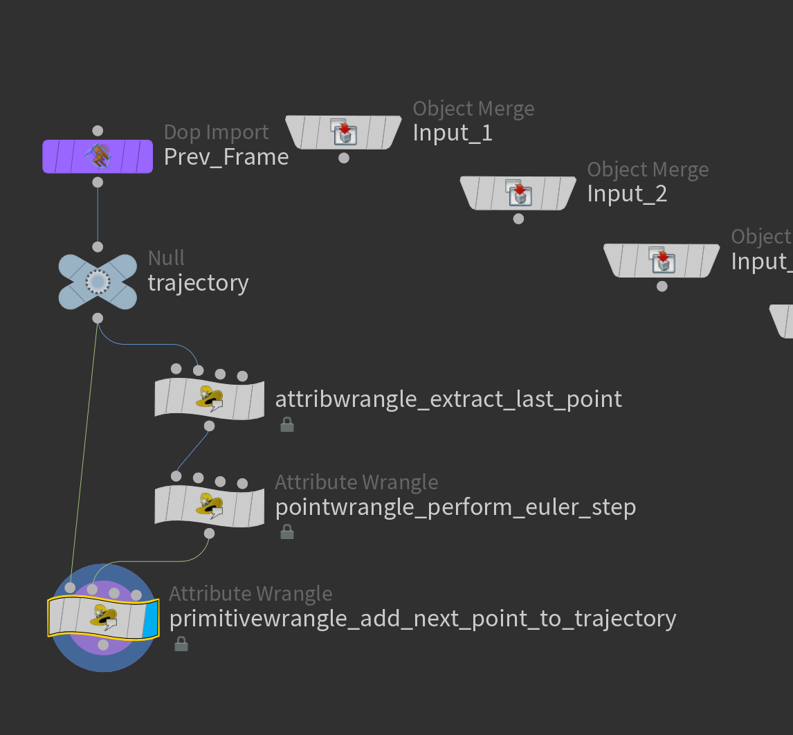
Here we use an Attribute Wrangle node (which ‘runs over’ detail) to extract the last point of the trajectory curve,
|
1 2 3 4 5 6 7 8 |
// The geometry of Input 1 is just one primitive (index 0) int curve = 0; // extract the point coordinates of the last point int points[] = primpoints(1,curve); int lastpoint = points[len(points)-1]; vector y_k = point(1,"P",lastpoint); // add the point to geometry of the current node addpoint(0,y_k); |
perform an Euler step (Point Wrangle node).
|
1 2 |
float h = .1; v@P += h*set(-v@P.y,v@P.x,0); |
and add this point to the trajectory curve (Primitive Wrangle node)
|
1 2 3 |
int i = @primnum; vector nexty = point(1,"P",i); addvertex(0,i,addpoint(0,nexty)); |
A more sophisticated method to solve differential equations is the so called Runge-Kutta method (RK4) It basically consists of 4 Euler steps and schematically this looks as follows:
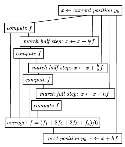
The scheme translates one to one into a Houdini network which then replaces the single Euler step node of the previous network:
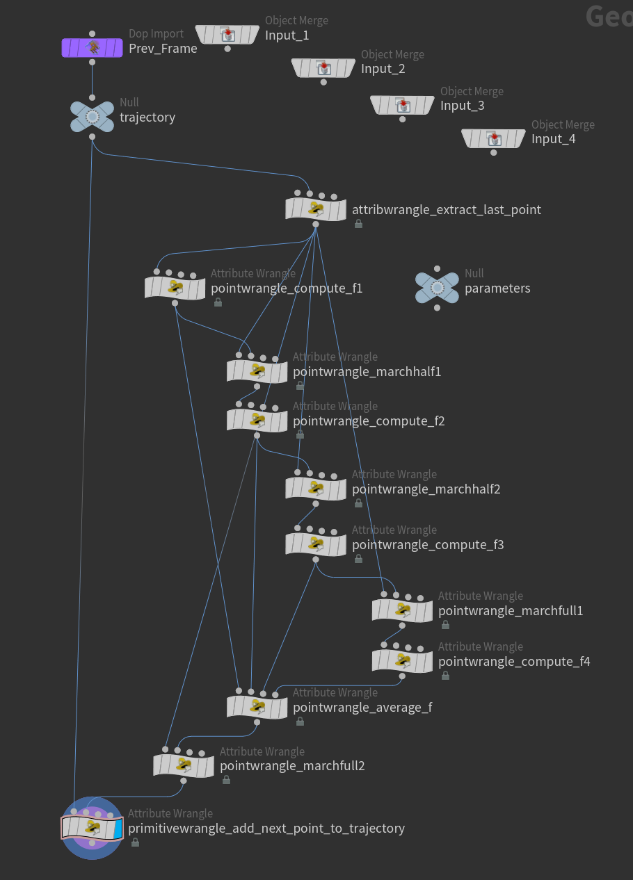
Moreover, we used here a null node to store the step size as a float parameter \(h\). The code of the single nodes is very simple: The pointwrangle_marchhalf1 contains e.g. just 3 lines
|
1 2 3 |
float delta = chf("../parameters/h")/2.; vector f = point(1,"f",@ptnum); v@P += delta*f; |
Similarly the ‘compute f’ nodes even consist of just one line
|
1 |
v@f = set(-v@P.y,v@P.x,0); |
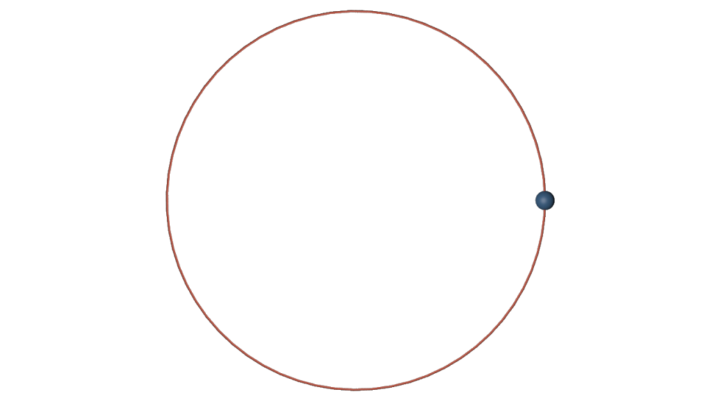
With the RK4 method we then obtain for \(h=.1\) a nice circle:
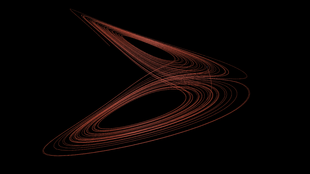
Let us apply this to the Lorenz attractor. We only have to change \(f\). We do this by creating a String parameter ‘code’ (multiline, VEX) in the parameters node.
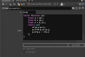
The code written there then can be imported in wrangle nodes by inserting <code>chs("../parameters/code") at the start of the ‘VEXpression’ field. E.g.
|
1 2 |
`chs("../parameters/code")` v@f = f(v@P); |
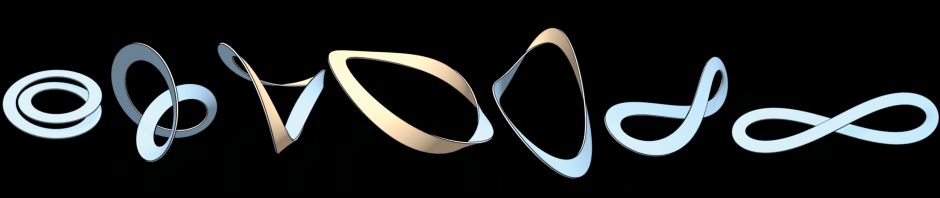
Here how the result then may look like:
The motion of a particle of charge \(q\) in a magnetic field \(B\colon \mathbb R^3 \to \mathbb R^3\) is given by a solution \(\gamma\colon \mathbb R \to \mathbb R^3\) of the second order ODE\[\gamma^{\prime\prime}(t) = q\,\gamma^\prime(t)\times B(\gamma(t)).\]Details can be found various internet pages and articles, as e.g. the Wikipedia article on Lorentz force or this article on the motion in constant and uniform fields.
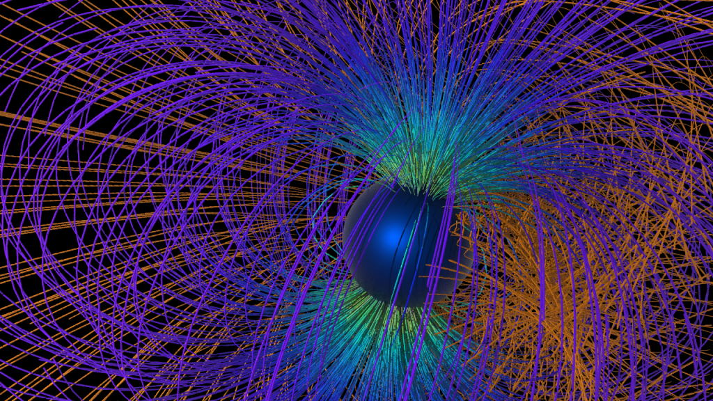
Homework (due 8 May). Modify the network such that it computes the trajectory of a charged particle moving in the field of a magnetic dipole. Therefore change the RK4 solver such that it operates on a float[] point attribute \(y\) (instead of the point positions), reduce the second order ODE to a first order ODE (on \(\mathbb R^6\)) and solve it.
Further one can use a Scatter node to generate particles equally distributed on a given geometry. Here a picture of 500 particles (with constant initial velocity) shot at a magnetic dipole.