DDG2018

The Biot-Savart formula provides for a given set of curves \(\gamma = (\gamma_1,\ldots,\gamma_m)\) a divergence-free velocity field whose vorticity is concentrated along these curves. This led to a simple algorithm to model fluids on entire \(\mathbb R^3\). Here we present a way to treat obstacles.

Let \(\sigma\) be the boundary surface of an obstacle \(M\). Since the fluid cannot penetrate \(M\) the velocity field is tangent to \(\Sigma\). So we are searching for a divergence-free vector field \(u\) that is tangent to \(\Sigma\) and still has the correct vorticity. This amounts to solving a boundary value problem.

The Biot-Savart field \(u_{\gamma}\colon \mathbb R^3 \to \mathbb R^3\) (always smoothed a bit) is not tangent but has already the correct vorticity. Now if \(u_{\sigma}\colon \mathbb R^3 \setminus M \to \mathbb R^3\) is a divergence-free curl-free field and has the same normal component as \(u_{\gamma}\), then \(u_{\gamma} – u_\Sigma\) is tangent to \(\Sigma\) and still has the correct vorticity, i.e.\[u=u_{\gamma}-u_\Sigma\]solves the boundary value problem.

Though we cannot solve exactly for \(u_\Sigma\), we can approximate it.

Let \(\Sigma\) be a polygonal surface and consider its cells as smoke rings, \(\eta = (\eta_1,\ldots,\eta_n)\). Then we can compute strengths \(\Gamma_1,\ldots,\Gamma_n\) such that the flux of the Biot-Savart field \(u_\eta\) of \(\eta\) through each facet of \(\Sigma\) equals the the flux of \(u_\gamma\). This can be done by solving the following quadratic linear system:\[\sum_{i=0}^n\mathrm{flux}_{\eta_i}(u_{\eta_j})\Gamma_j = \mathrm{flux}_{\eta_i}(u_\gamma),\quad i,j\in \{1,\ldots,n\}.\]Since \(\eta_i\) are polygons the values \(\mathrm{flux}_{\eta_i}(u_{\eta_j})\) can be computed directly as a sum of ‘edge fluxes’,\[\mathrm{flux}_{\eta_i}(u_{\eta_j}) = \sum_{e\in \eta_i} \sum_{\tilde e\in\eta_j} \mathrm{edgeflux}(e,\tilde e),\]and there is an explicit formula to compute \(\mathrm{edgeflux}(e,\tilde e)\), which is implemented as method edge_flux in the following .h-file. Details can be found e.g. in the Steffen Weissmann’s thesis. How to include .h-files is explained here.

In this exercise we will use this technique to change a static constant field \(u_c = X \in \mathbb R^3\) to a field \(u\) that flows around \(\Sigma\).

The flux though a facet \(\varphi_i\) of \(\Sigma\) is then equal to the product of the area vector \(A\) and the vector \(X\): If \(\eta_i = \partial \varphi_i= (p_1,\ldots,p_k)\),\[\mathrm{flux}_{\eta_i}(u_c) = \langle A_i,X\rangle, \quad A_i = \tfrac{1}{2}\sum_{j=0}^k p_j\times p_{j+1}.\]Thus we have \(u = u_c – \sum_{i}\Gamma_i u_{\eta_i}\), where \(u_{\eta_i}\) denotes the smoothed Biot-Savart field and the coefficients \(\Gamma_i\) solve the following linear system\[\sum_{i=0}^n\mathrm{flux}_{\eta_i}(u_{\eta_j})\Gamma_j = \langle A_i,X\rangle.\]

All the fluxes can be computed in VEX. To solve the linear system we finally need Python. Therefore we can use a Python node with the following code

Here fluxmatrix is a global float[] attribute that contains the fluxes \(\mathrm{flux}_{\eta_i}(u_{\eta_j})\), i.e.\[\mathtt{fluxmatrix[i*n + j]} =\mathrm{flux}_{\eta_i}(u_{\eta_j})\]and A_X is a global float[] attribute containing the fluxes of \(u_c\), i.e.\[\mathtt{A\_ X[i]} =\langle A_i,X\rangle.\]

Homework (due 17 July). Write a network that, for a given vector \(X\in\mathbb R^3\) and a given surface \(\Sigma\) computes the corresponding velocity field \(u\). Visualize the integral curves of \(u\).

The velocity field of a fluid in \(\mathbb R^3\) (at rest at infinity) can be reconstructed from the vorticity by the Biot-Savart formula. Let us assume a fluid with vorticity concentrated along a filaments: Given a curve \(\gamma\colon \mathbb S^1 \to \mathbb R^3\) and \(a>0\), then the corresponding (smoothed) Biot-Savart field \(u_a\colon \mathbb R^3\to \mathbb R^3\) of \(\gamma\) (with smoothing parameter \(a\)) is given by \[u_a(p) = \frac{1}{4\pi}\int_{\mathbb S^1} \frac{(\gamma-p)\times d\gamma}{\sqrt{a^2+ |\gamma-p|^2}^3}.\]The field \(u_a\) is divergence-free with vorticity \(w_a=\mathrm{curl}\, u_a\) concentrated in a tube of radius \(a\) along \(\gamma\). \(w_a\) is obtained from \(\gamma\) by convolution with a certain smoothing kernel.

For \(a\to 0_+\) the vorticity \(w_a\) tends to the current given by integration over \(\gamma\): For \(v\colon \mathbb R^3 \to \mathbb R^3\) smooth with compact support, \[\lim_{a\to 0_+} \int_{\mathbb R^3} \langle v,w_a\rangle = \int_{\mathbb S^1} \langle v\circ\gamma,d\gamma\rangle.\]In the following we will suppress the dependency on the smoothing parameter \(a\).

The vorticity is frozen in the fluid, i.e. \(\dot w + [u,w] = 0\). By the Biot-Savart formula we can reconstruct the velocity of the fluid only from its vorticity, this offers the possibility to approximate the whole fluid by advection of its vortex filaments, i.e. we just have to solve\[\dot\gamma = u\circ\gamma.\]This simple algorithm already enables us to reproduce certain phenomena – like e.g. leapfrogging smoke rings as shown in the picture above. All we need to know is the Biot-Savart field of a closed polygon.

Fortunately the Biot-Savart formula be explicitly integrated along straight edges: Given an (oriented) edge \(e\) parametrized by \(\eta\colon [0,1]\to \mathbb R^3\) with \(\eta(t) = q_1 + t(q_2-q_1)\), then \[u_e(p) =\frac{1}{4\pi}\int_0^1 \frac{(\eta-p)\times d\eta}{\sqrt{a^2+ |\eta-p|^2}^3}.\]Note that \(\eta^\prime = q_2-q_1\) and thus \((\eta-p)\times \eta^\prime = (q_1-p)\times (q_2-q_1)\) are constant. We have\[\frac{(\eta-p)\times \eta^\prime}{\sqrt{a^2+ |\eta-p|^2}^3} =\Bigl(\frac{\langle \eta – p, \eta^\prime\rangle \, (\eta – p)\times \eta^\prime}{\bigl(|\eta^\prime|^2 a^2 + |(\eta – p)\times\eta^\prime|^2\bigr)\sqrt{a^2 + |\eta – p|^2}}\Bigr)^\prime,\]where \((.)^\prime\) denotes the derivative with respect to the parameter \(t\). Thus we obtain an explicit formula for \(u_e\) in terms of the start and end point \(q_1\) and \(q_2\) of \(e\).

So, given a polygon \(\gamma\) we obtain the corresponding Biot-Savart field \(u\) by summing over the oriented edges of \(\gamma\). The picture bleow shows the integral curves of the Biot-Savart field of a discrete \(\gamma\) together with level sets of the solid angle function of \(\gamma\).

As expected the integral curves intersect the level sets orthogonally.

In general, given a set of discrete curves \(\gamma^1, \ldots, \gamma^m\), then we have \[u(p) = \sum_{\textit{edge e}} u_e(p),\]where \(u_e\) denotes the Biot-Savart field of the edge \(e\) and the sum runs over all (positively oriented) edges \(e\) in \(\gamma^1,\ldots,\gamma^m\).

Homework (due 3 July). Write a network that, for a given set of polygons, advects the vertices of the polygons by their own Biot-Savart field. Use a Runge-Kutta scheme and make it possible to move particles with the fluid.

Let \(\gamma\colon \mathbb S^1 \to \mathbb R^3\) be a closed space curve and \(m\in\mathbb R^3\setminus \gamma(\mathbb S^1)\). The solid angle \(\Omega_{\gamma}(m)\) of \(\gamma\) subtended to the point \(m\) is defined as the (signed) spherical area enclosed by the projection \(\hat\gamma\) of \(\gamma\) to the unit sphere with center \(m\),\[\hat\gamma = \frac{\gamma-m}{|\gamma – m|}+m\] Note that the spherical area is defined only up to addition of an integral multiple of \(4\pi\). Hence \(\Omega_\gamma\) is a well-defined angle-valued map\[\Omega_\gamma\colon \mathbb R^3\setminus \gamma(\mathbb S^1) \to \mathbb R/4\pi \mathbb Z.\]The solid angle of a closed discrete space curve \(\gamma\colon \mathbb Z/n\mathbb Z \to \mathbb R^3\) is then defined by the solid angle of the closed polygon \(P_\gamma\) corresponding to \(\gamma\).

The polygon \(P_\gamma\) projects to the spherical polygon corresponding to \((\gamma-m)/|\gamma – m|+m\). Since translations do not change area we are left with the problem to compute the (signed) area of a spherical polygon in the unit sphere \(\mathbb S^2\subset \mathbb R^3\). This can be done e.g. by the Gauss-Bonnet Theorem: Let \(\hat\gamma \colon \mathbb Z/n\mathbb Z \to \mathbb S^2\). Let \(\mathbb D\) be the unit disk in \(\mathbb R^2\) and \(f\colon \mathbb D \to \mathbb S^2\) be a regular surface such that \(f|_{\mathbb S^1}\) parametrizes the spherical polygon corresponding to \(\hat\gamma\). Then, since the all edges are geodesics and \(\chi_M = 1\), we get\[\mathrm{Area}(f) = \int_D f^\ast d\mathrm{vol}_{\mathbb S^2} = 2\pi – \sum_i\kappa_i,\]where \(\kappa_i\) denote the kink angles of the spherical polygon. \(\kappa\) can be computed from the discrete spherical curve \(\hat\gamma\).

Another, more elementary way to compute the area is to use a triangulation. Therefore choose a point \(c\in\mathbb S^2\setminus\{-\hat\gamma_0,\ldots,\hat\gamma_{n-1}\) and connect each vertex of \(\hat\gamma\) to \(c\) by the great circle arc of length \(< \pi\). Note that the points \(c\), \(\gamma_i\) and \(\gamma_{i+1}\) lie in an open hemisphere. We obtain a triangulated disk with \(n\) triangles of the form \(\triangle_i = (c,\hat\gamma_i,\hat\gamma_{i+1})\) each of which is contained in an open hemisphere. The area enclosed by \(\hat\gamma\) is then just the sum of the areas of the spherical triangles \(\triangle_i\) for which we have an elementary formula: Given a positively oriented spherical triangle \(\triangle = (a_0,a_1,a_2) \in \mathbb S^2\) contained in an open hemisphere, then the area\[\mathrm{Area}(\triangle) = \sum_{i=0}^2 \alpha_i – \pi,\]where \(\alpha_i\in (0,\pi)\) denotes the interior angle at \(a_i\). To see this look at the lunes \(\lambda_i\) generated by \(a_{i-1}\), \(a_{i}\) and \(a_{i+1}\).

Then the union of \(\lambda_0\), \(\lambda_1\) and \(\lambda_2\) covers half of the sphere. Thus the area of their union is \(2\pi\). Each lune itself has area \(2\alpha_i\). Thus we get \(2 \sum_{i=0}^2 \alpha_i = 2\pi + 2\mathrm{Area}(\triangle)\). If the original triangle was negatively oriented we just flip the sign.

Yet another way to compute the area of an oriented spherical triangle is to use the following relation between parallel transport and curvature: Let \(M\) be a Riemannian surface with boundary \(\partial M\), let \(J\) denote the complex structure of \(M\) (i.e. the 90 degree rotation in \(TM\)) and let \(P_\eta\) denote the parallel transport along a curve \(\eta\) in \(M\). Then\[P_{\partial M} = e^{J\int_M K\,d\mathrm{vol}_M}.\] In particular, if \(K=1\), we get\[P_{\partial M} = e^{J\mathrm{Area}(M)}.\]The advantage of this version is that is also applies to singular triangles.

Consider two point \(p\) and \(q\) on \(\mathbb S^2 \subset \mathbb R^3 \cong \mathrm{Im}\,\mathbb H\). If \(q\neq -p\), then there is a unique shortest great circle arc \(\eta\colon [0,1]\to \mathbb S^2\) connecting them. So we can speak of \(P_{p,q}\). Actually \(P_{p,q}\) can be written down by quaternions:\[P_{p,q}(X) = \psi_{p,q} X \psi_{p,q}^{-1}.\]Let us verify that \(\psi_{p,q} = q(p+q)\): The quaternion \(p+q\) represents a \(180\) rotation \(R_1\) around the vector \(p+q\). Similarly, \(q\) represents a \(180\) degree rotation \(R_2\) around \(q\). Thus \(\psi_{p,q}\) representing the rotation \(R_2R_1\) restricts to an isometry \(T_p\mathbb S^2 \to T_q\mathbb S^2\) mapping \(\eta^\prime(0)\) to \(\eta^\prime(1)\). Since \(\eta\) is a geodesic, \(\eta^\prime\) is parallel.  The claim then follows since parallel transport is angle and orientation preserving.

The quaternion \(\psi_{p,q}\) is defined only up to a non-zero real multiple. Thus, if \(p=q\), then \(\psi_{p,q} = 1\). If \(p\neq q\), then \[\psi_{p,q} = 1+\tan(\mathrm{dist}(p,q)/2)\, N,\] where \(\mathrm{dist}(p,q)\) denotes the spherical distance of \(p\) and \(q\), i.e. the length of \(\eta\), and \(N\) denotes the normal of the great circle arc pointing to the left, i.e. \(N = J\eta^\prime(t)\) for some \(t\).

Now, let us consider the spherical triangle \(\triangle = (a_0,a_1,a_2)\). We have \[e^{J\mathrm{Area(\triangle)}} = P_{a_2,a_0}\circ P_{a_1,a_2}\circ P_{a_0,a_1}.\]

In quaternions this becomes\[\rho\,(1+\tan(\mathrm{Area}(\triangle)/2)a_0) = (1+\tan(\ell_1/2)n_1)(1+\tan(\ell_0/2)n_0)(1+\tan(\ell_2/2)n_2).\]Here \(\ell_i\) denotes the arc length and \(n_i\) the inward pointing normal of the great circle arc opposite to the point \(a_i\). We can multiply the equation from the right by the inverse of \(1+\tan(\ell_2/2)n_2\). This yields the following quaternionic equation\[\rho\,(1+\tan(\mathrm Area(\triangle)/2)a_0)(1-\tan(\ell_2/2)n_2) = (1+\tan(\ell_1/2)n_1)(1+\tan(\ell_0/2)n_0),\] where the real factor \(|1+\tan(\ell_2/2)n_2|^{-2}\) is absorbed into \(\rho\).

Sicne \(a_0\perp n_2\), taking now the real part on both sides of the quaternionic equation yields\[\rho = 1 – \tan(\ell_0/2)\tan(\ell_1/2)\langle n_0,n_1\rangle = 1 + \tan(\ell_0/2)\tan(\ell_1/2)\cos(\alpha_2).\]By taking the imaginary part on both sides of the quaternionic equation, we get\begin{gather*}\rho(\tan(\mathrm{Area}(\triangle)/2)a_0 – \tan(\ell_2/2)n_2 – \tan(\mathrm{Area}(\triangle)/2)\tan(\ell_2/2)a_0\times n_2)\\ = \tan(\ell_0/2)n_0 + \tan(\ell_1/2)n_1 – \tan(\ell_0/2)\tan(\ell_1/2)n_0\times n_1.\end{gather*} Moreover, \(a_0\perp n_1,n_2\) and \(n_0\times n_1 = \sin(\alpha_2) a_2\), where \(\alpha_i\) denotes the oriented interior angle at \(a_i\). If we now build the scalar product with \(a_0\), we obtain \[\rho\tan(\mathrm{Area}(\triangle)/2) = \tan(\ell_0/2)\bigl(\langle a_0,n_0\rangle – \tan(\ell_1/2)\sin(\alpha_2)\cos(\ell_1)\bigr).\]With \(\sin(\ell_0)\langle n_0,a_0\rangle = \langle a_1\times a_2, a_0\rangle = \sin(\ell_0)\sin(\ell_1)\sin(\alpha_2)\) we then get\begin{gather*}\langle a_0,n_0\rangle – \tan(\ell_1/2)\sin(\alpha_2)\cos(\ell_1) = \sin(\alpha_2)\bigl(\sin(\ell_1)- \tan(\ell_1/2)\cos(\ell_1)\bigr) \\ = \sin(\alpha_2)\bigl(2\sin(\ell_1/2)\cos(\ell_1/2) – \tan(\ell_1/2)(\cos^2(\ell_1/2) – \sin^2(\ell_1/2)\bigr) \\ = \sin(\alpha_2)\tan(\ell_1/2)\bigl(2\cos^2(\ell_1/2) – (\cos^2(\ell_1/2)-\sin^2(\ell_1/2)\bigr) = \sin(\alpha_2)\tan(\ell_1/2).\end{gather*}Hence we get\[\tan(\mathrm{Area}(\triangle)/2) = \frac{1}{\rho}\tan(\ell_0/2)\tan(\ell_1/2)\sin(\alpha_2) = \frac{\tan(\ell_0/2)\tan(\ell_1/2)\sin(\alpha_2)}{1 + \tan(\ell_0/2)\tan(\ell_1/2)\cos(\alpha_2)}.\]Moreover, note that the tangents are given by purely algebraic formulas: Since \(\tan(\theta/2) = \sin(\theta)/(1+\cos(\theta))\) we have \[\tan(\ell_0/2) = \frac{|a_0-\langle a_0,a_2\rangle a_2|}{1 + \langle a_0,a_2\rangle},\quad \tan(\ell_1/2) = \frac{|a_1-\langle a_1,a_2\rangle a_2|}{1 + \langle a_1,a_2\rangle}.\]Moreover, \[\cos(\alpha_2)\sin(\ell_0)\sin(\ell_1) =  \bigl\langle a_0 – \langle a_0,a_2\rangle a_2, a_1 – \langle a_1,a_2\rangle a_2\bigr\rangle = \langle a_0,a_1\rangle – \langle a_0,a_2\rangle\langle a_2,a_1\rangle\] and with \(\det(a_0,a_1,a_2)=\sin(\ell_0)\sin(\ell_1)\sin(\alpha_2)\) we get\[\alpha_2 = \mathtt{atan2}(\det(a_0,a_1,a_2),\langle a_0,a_1\rangle – \langle a_0,a_2\rangle\langle a_2,a_1\rangle).\]

Now, given a closed discrete space curve \(\gamma\) we can compute the solid angle \(\Omega_\gamma(m)\). But how can we visualize the solid angle in Houdini?

A convenient way to do this is to compute the solid angle for the voxel centers of a volume surrounding \(\gamma\) and then use a convert volume node to extract the zero level set of \(\Omega_\gamma\). Here is how such a network may look like.

Volume wrangle nodes work quite similar to attribute wrangle nodes. Here the code block of the node volumewrangle1 in the network above:

The method to compute the solid angle is contained in a string parameter of a null node ‘sphericalarea’ and imported at the beginning of the block. The volume is initialized with the name Omega (the string specified in the name field of the volume node). The values then can be accessed and set via f@Omega. Note that volumes also have a boundary type which here should be set to ‘streak’. You find this parameter in the properties tab of the Volume node. Here is what we get.

The artifacts in the picture above are due to \(4\pi\) jumps , which cannot be handled by the convert volume node. We can get rid of them by applying a \(4\pi\)-periodic function as e.g. \(x\mapsto \sin(x/2)\). Only that the zero set now corresponds to \(\Omega_\gamma^{-1}(0)\cup \Omega_\gamma^{-1}(\pi)\). We can remove the  \(\Omega_\gamma^{-1}(\pi)\) part as follows: Create a second volume to store the values of \(\cos(\Omega_\gamma/2)\). From this we extract a second surface and use a boolean intersect node to cut of everything inside the second surface.

Homework (due 26 June). Write a network that computes for a given discrete space curve the level sets of the solid angle.

In class you defined the Darboux transformation \(\eta\colon \mathbb R\to \mathbb R^3\) of a smooth space curve \(\gamma\colon \mathbb R\to \mathbb R^3\). By construction, the distance between corresponding points is constant. Or phrased differently, there is \(S\colon \mathbb R \to \mathbb S^2 \subset \mathbb R^3\) such that \[\eta=\gamma + \ell S.\]Moreover, you proved that Darboux transformations preserve arc length. This led to the following definition of the discrete Darboux transformation: A discrete space curve \(\eta\colon \mathbb Z  \to \mathbb R^3\) is called a Darboux transformation of a discrete space curve \(\gamma\colon \mathbb Z \to \mathbb R^3\) with rod length \(\ell\) and twist \(r\) if \[\eta_j = \gamma_j + \ell S_j,\] where \(S\colon \mathbb Z \to \mathbb S^2\) satisfies\[S_{j+1} =(r+\ell S_j-v_jT_j)S_j(r+\ell S_j-v_jT_j)^{-1}.\]Here \(v_jT_j = \gamma_{j+1}-\gamma_j\) with \(v_j=|\gamma_{j+1}-\gamma_j|\). Compare also with this post from 2013.

The discrete Darboux transformation is easily implemented – given a discrete space curve \(\gamma=(\gamma_0,\ldots,\gamma_{n-1})\), a point \(p\in\mathbb R^3\) and \(r\in \mathbb R\), then we obtain a discrete Darboux transformation \(\eta\) of rod length \(\ell := |\gamma_0 – p|\) and twist \(r\) starting at \(p\) (\(\eta_0 = p\)) as follows:

1. Set \(S_0 := (\eta_0 – \gamma_0)/\ell\),
2. iteratively compute \(S\), and
3. define \(\eta_j := \gamma_j + \ell S_j\).

As we want to play around with the Darboux transformation we want to have control over the initial data \(p\) and \(r\). The parameter \(r\) can be just given as a node parameter. The initial point \(p\) can just be given by a geometry containing just a single point which is then made draggable by an edit node. Here is how such a network could look like:

In general, a Darboux transformation of a closed discrete space curve \(\gamma \colon \mathbb Z/n\mathbb Z \to \mathbb R^3\) is not closed. Though, for given \(\ell\) and \(r\) the map \(M_{\ell,r} \colon \mathbb R^3 \to \mathbb R^3\) sending the initial rod direction \(S_0\) to the end rod direction \(S_n\) is a Moebius transformation, a generic discrete space curve will have exactly two closed Darboux transformations corresponding to the fixed points of \(M_{\ell,r}\). These points could be computed directly from \(M_{\ell,r}\). Unfortunately if we try to compute \(M_{\ell,r}\) we run into numerical problems . Fortunately, we quickly converge to a fixed point when running around \(\gamma\) several times (always computing a new Darboux transformation starting from the end of the previous).

Affectively this amounts to applying \(M_{\ell,r}\) several times but turns out to be numerically stable and quite fast. So we can compute a closed Darboux transformation of a discrete space curve \(\gamma\colon \mathbb Z/n\mathbb Z \to \mathbb R^3\) with rod length \(\ell\) and twist \(r\) as follows:

1. Compute for sufficiently large \(m \in\mathbb N\) the direction \(\tilde S_{mn}\) starting from some initial rod direction \(S_0\in\mathbb S^2\),
2. Compute the Darboux transformation \(\eta\) starting at \(\gamma_0+\ell \tilde S_{mn}\).

Similarly, a second fixed point is found when running \(\gamma\) backwards (iterating \(M_{\ell,r}^{-1}\)).

Homework (due 19 June). Write a digital asset which computes for a closed discrete space curve a closed Darboux transformation with rod length \(\ell\) and twist \(r\). Use a checkbox to specify whether to iterate forward of backward.

The goal of this post is to implement certain time-continuous flows on discrete space curves. By a time-continuous flow of a closed discrete space curve \(\gamma\colon \mathbb Z/n\mathbb Z \to \mathbb R^3\) we mean the continuous solution of an equation\[\dot\gamma = X(\gamma)\]Here \(X\) is vector field on the space of discrete curves, i.e. a map that assigns to a curve \(\gamma\) with \(n\) vertices a sequence \(X(\gamma)\colon \mathbb Z/n\mathbb Z \to \mathbb R^3\).

In this post we will focus on the Möbius tangent flow, which is a discrete analogue of the continuous tangent flow \(\dot\gamma = \gamma^\prime\), and a discrete analogue of the continuous vortex filament flow \(\dot\gamma = \gamma^\prime \times \gamma^{\prime\prime}\). Here \((.)^\prime\) denotes the derivative with respect to arclength.

While in the continuous setup the tangent flow is trivial (it just acts by reparametrization), the discrete tangent flow will change the shape of the polygon.

Given a closed discrete space curve with \(n\) vertices, i.e. \(\gamma\colon \mathbb Z/n\mathbb Z \to \mathbb R^3\), then for each edge we have an edge vector \[S_i = \gamma_{i+1}-\gamma_i\]This provides a canonical (unit) tangent vector along each edge. Though at a vertex itself there is no obvious choice of a tangent vector – there is a whole interval of candidates.

E.g. one reasonable choice for \(T_i\) could be the angle bisector between \(S_{i-1}\) and \(S_i\), i.e. \[\Bigl(\tfrac{S_{i-1}}{|S_{i-1}|}+\tfrac{S_i}{|S_i|}\Bigr)/\Bigl|\tfrac{S_{i-1}}{|S_{i-1}|}+\tfrac{S_i}{|S_i|}\Bigr|\]Another possible definition of \(T\),  leading to a much more stable and, in fact, Möbius invariant flow is given by the harmonic mean of \(S_{i-1}\) and \(S_i\), i.e.\[T_i=\frac{|S_{i}|^2S_{i-1} + |S_{i-1}|^2S_i}{|S_{i-1}+S_i|^2}\]Note that for arc length parametrized \(\gamma\), i.e. \(|S_i| = 1\), both definitions coincide. Details can be found e.g. in Tim Hoffmann’s lecture on Discrete Differential Geometry of Curves and Surfaces or Alexander Bobenko’s script on Discrete Differential Geometry.

Mainly the flow \(\dot\gamma = T\) just shifts the vertices along the curve. Though if we run the simulation at high speed the shape of the curve changes essentially, as shown in the following video.

We observe loops traveling along the curve, interacting when passing each other while basically keeping their shape. This kind of phenomenon hints at a connection to soliton theory.

Another flow related to soliton theory is the vortex filament flow. It describes how vortex filaments move and is related to the cubic non-linear Schrödinger equation – an equation well-known to soliton theorists.

To motivate the discrete vortex filament flow let us look at the continuous equation and assume for a second that we are dealing with a Frenet curve, i.e. \(\gamma^{\prime\prime} \neq 0\). Here again \((.)^\prime\) denotes the derivative with respect to arc length. Then with \(T= \gamma^\prime\), \(N = \gamma^{\prime\prime}/|\gamma^{\prime\prime}|\) and \(B =T\times N\) we get \(\gamma^{\prime\prime}= \kappa N\) and the vortex filament flow becomes\[\dot\gamma = \kappa B\]The function \(\kappa\) is the so called Frenet curvature of \(\gamma\) and equals the the inverse radius of the osculating circle.

Certainly a discrete curve is not a Frenet curve. Though unless \(S_{i-1}\) and \(S_i\) are parallel there is an osculating plane and a corresponding normal \(B_i\) perpendicular to that plane which was already used in a previous post to define the discrete Frenet frame. But what is a discrete Frenet curvature? Again there is no canonical choice and several choices are presented in the scripts mentioned above. We will just stick here to the definition using vertex osculating circles as in Tim Hoffmann’s paper, i.e.\[\kappa_i = \frac{2\sin(\alpha_i)}{|S_{i-1}+S_i|}\]where \(\alpha_i\) denotes the angle between \(S_{i-1}\) and \(S_i\). Thus we get\[k_iB_i = \frac{2\,S_{i-1}\times S_i}{|S_{i-1}||S_{i-1}+S_{i}||S_i|}\]

The surface swept out by the vortex filament flow are called Hashimoto surfaces. They can be easily visualized with help of Houdini’s trail node. The point attribute @Alpha controls the alpha channel of the point color and can be used to fade out the trail. Here is a picture how such a surface can look like.

Homework (due 29 May). Use your Runge-Kutta solver to compute the Möbius tangent and vortex filament flow of a prescribed closed discrete space curve.

Update: Albert has written a digital asset which makes it possible to plot how certain quantities (stored as detail attribute) evolve under the flow.

Homework (due 5 June). Plot the length, the area (projected to a plane) and the energy of a curve (with constant edge length) moving under the tangent and the vortex filament flow. Here energy is defined by \(E = \frac{2}{\ell}\sum_{i}\log(1+\tan^2(\frac{\alpha_i}{2}))\), where \(\ell\) denotes the edge length.

Under a discrete space curve \(\gamma\) we understand a (finite or periodic) sequence \(\gamma_i\) of points in \(\mathbb R^3\). The \(i\)-th edge vector is then denoted by \(e_i = \gamma_{i+1} – \gamma_i\) and has length \(\ell_i = |e_i|\). If \(\ell_i\neq 0 \) for all \(i\) we call \(\gamma\) regular and define the tangent vector \(T_i=e_i/\ell_i\).

A frame for \(\gamma\) is then an assignment of a positively oriented orthonormal basis \(T_i,N_i,B_i\) to each edge \(e_i\) of \(\gamma\), i.e. to each edge it assigns a rotation \[\sigma_i = (T_i,N_i,B_i) \in \mathrm{SO}(3).\]

Quaternions. The quaternions, denoted \(\mathbb H\), are a number system similar to the complex numbers but with \(3\) linearly independent imaginary units \(\mathbf i, \mathbf j,\mathbf k\): A quaternion \(q \in \mathbb H\) is a number of the form\[q = w + x\,\mathbf i + y\,\mathbf j + z\,\mathbf k, \quad w,x,y,z\in \mathbb R.\]In analogy to the complex numbers we define \(\mathrm{Re}(q) := w\) (real part of \(q\)), \(\mathrm{Im}(q) := x\mathbf i + y\mathbf j + z\mathbf k\) (imaginary part of \(q\)) and \(\bar q = \mathrm{Re}(q)-\mathrm{Im}(q)\) (conjugate of \(q\)).

The quaternionic multiplication is determined by the following multiplication rules:\[\mathbf i^2 = \mathbf j^2 = \mathbf k^2 = -1, \quad \mathbf{i\,j}=\mathbf{k}= -\mathbf{j\,i},\quad \mathbf{j\,k}=\mathbf{i}=-\mathbf{k\,j},\quad \mathbf{k\,i}=\mathbf{j}=-\mathbf{i\,k}.\]

In Houdini the quaternionic multiplication is implemented by the VEX function

• vector4 qmultiply(vector4 q1, vector4 q2)

As quaternions provide a convenient way to represent rotations, they are well-known in Computer Graphics. In Houdini they appear as \(4\)-vectors:\[\mathbb R^4 \ni \mathbf (w,x,y,z) \longleftrightarrow w + x\,\mathbf i + y\,\mathbf j + z\,\mathbf k \in \mathbb H.\]So what has this to do with rotations in Euclidean \(3\)-space? Let us identify \(\mathbb R^3\) with the purely imaginary quaternions \(\mathrm{Im}\, \mathbb H = \mathrm{span}_{\mathbb R}\{\mathbf i,\mathbf j,\mathbf k\}\)\[\mathbb R^3 \ni \mathbf (x,y,z) \longleftrightarrow x\,\mathbf i + y\,\mathbf j + z\,\mathbf k \in \mathrm{Im}\,\mathbb H.\]Let \(q = \cos(\tfrac{\alpha}{2}) + \sin(\tfrac{\alpha}{2})\mathbf a\) with \(\alpha \in \mathbb R\) and \(\mathbf a \in \mathbb S^2 \subset \mathrm{Im}\,\mathbb H\), then the map \(R_q\colon \mathbb R^3 \to \mathbb R^3\) given by\[\mathbf v \mapsto q\mathbf v \bar q\]is a (positive) rotation by the angle \(\alpha\) around the vector \(\mathbf a\). If one is used to quaternionic algebra this is easy to see. We skip this here. A proof can be found e.g. in the DDG 2016 blog.

The maps \((\alpha,\mathbf v)\mapsto \cos(\tfrac{\alpha}{2}) + \sin(\tfrac{\alpha}{2})\mathbf v\) and \((q,\mathbf v) \mapsto R_q(\mathbf v)\) are built into Houdini by the following VEX functions:

• vector4 quaternion(float angle, vector axis)
• vector qrotate(vector4 quaternion, vector a)

Remark. It is an easy exercise to check that \(\overline{q_1q_2} = \overline{q_2}\,\overline{q_1}\). Thus \(\mathbb S^3 = \{q\in\mathbb H \mid |q|^2 = \bar q q = 1\}\) forms a group. Moreover, \(R_{q_1}\circ R_{q_2} = R_{q_1q_2}\), i.e. the map \(\mathbb S^3 \to \mathrm{SO}(3)\), \(q\mapsto R_q\) is a group homomorphism. Actually it is a \(2\)-sheeted covering, \(R_{q} = R_{-q}\).

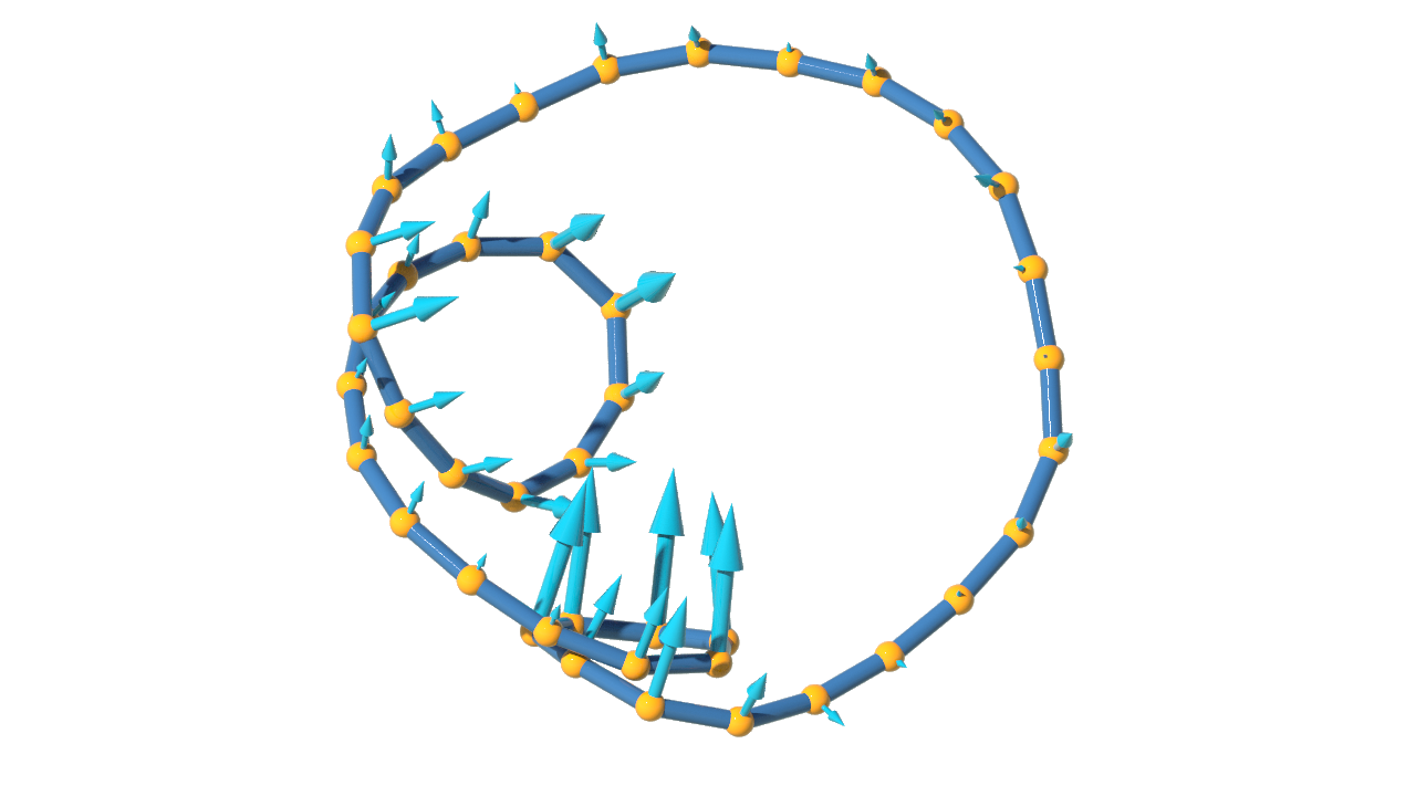
Quaternionic frames and the Copy Stamp node. Let \(\gamma\) be a regular discrete space curve. A discrete frame is a map which assigns to each edge \(e_i\) of \(\gamma\) a rotation \(\sigma_i \in \mathrm{SO}(3)\) such that\[T_i = \sigma_i\left(\begin{smallmatrix}1\\0\\0\end{smallmatrix}\right),\quad N_i = \sigma_i\left(\begin{smallmatrix}0\\1\\0\end{smallmatrix}\right), \quad B_i = \sigma_i\left(\begin{smallmatrix}0\\0\\1\end{smallmatrix}\right)\]A quaternionic frame \(\psi\) is then a lift of \(\sigma\), i.e. for all \(i\) we have \(\psi_i\in\mathbb S^3\) such that \(\sigma_i = R_{\psi_i}\). In particular, we have\[T_i = \psi_i\,\mathbf i\,\bar{\psi_i}, \quad N_i = \psi_i\,\mathbf j\,\bar{\psi_i}, \quad B_i = \psi_i\,\mathbf k\,\bar{\psi_i}.\]For the visualization we can use Houdini’s Copy Stamp node. Looking at its Copying and instancing point attributes we find that this node can handle quaternionic frames out of the box (there appearing as the point attribute @orient). Moreover we can specify for each point a scale factor (point attribute @pscale).

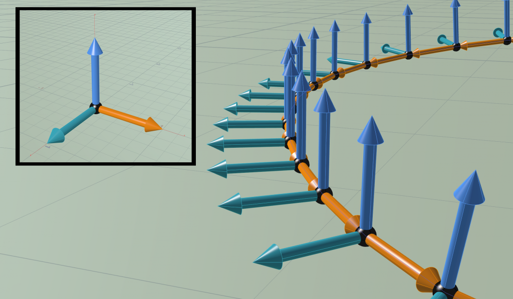
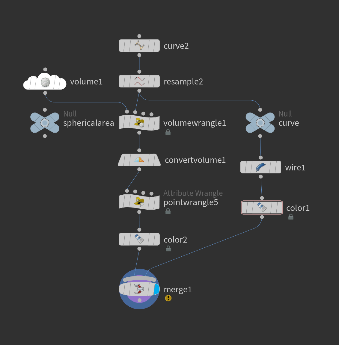
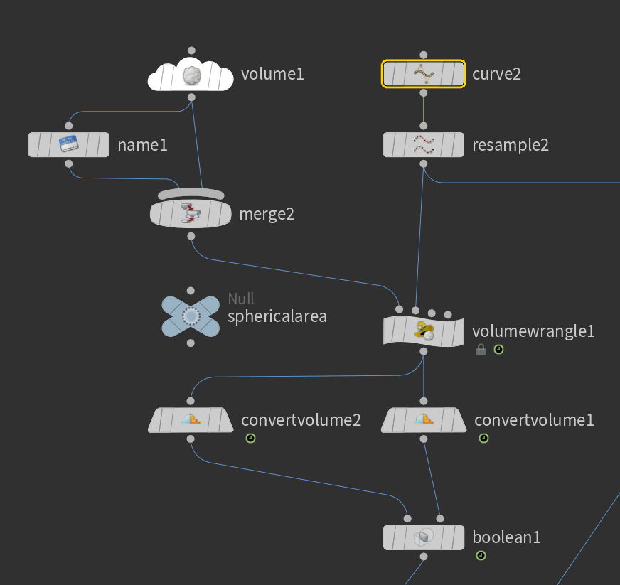
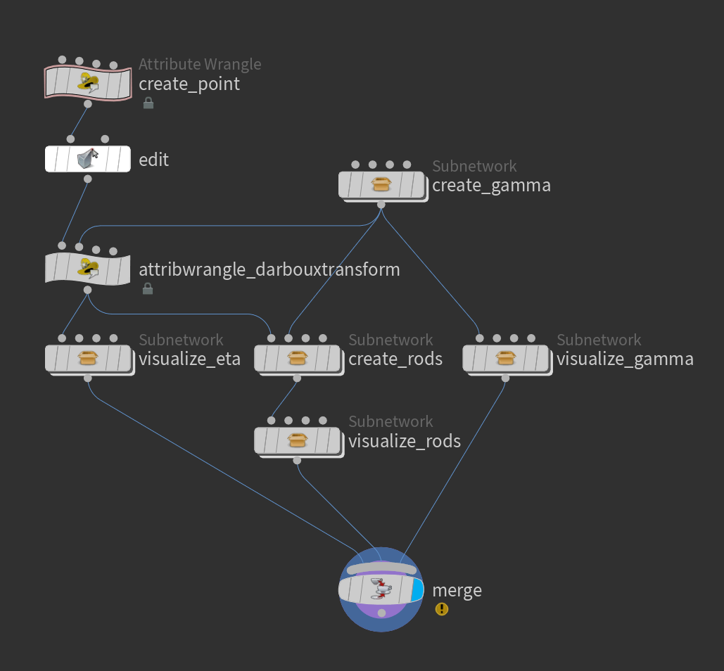
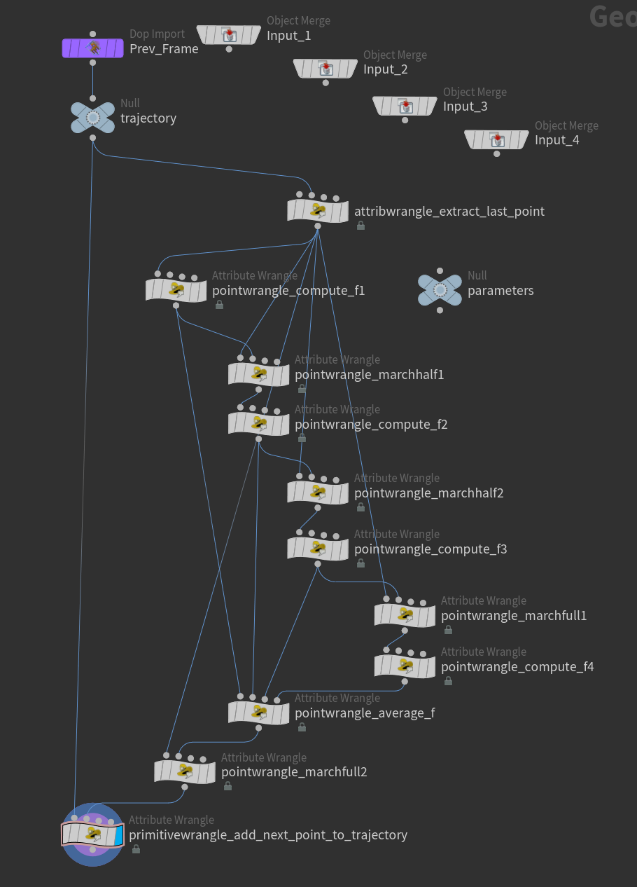
The picture below shows how such a network could look like.

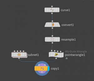
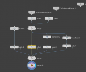
The subnet1 node merges colored tubes and a sphere to visualize the standard frame. The network is shown in the picture below.

So far the VEX code contained in pointwrangle1 produces just some arbitrary frame:

The method dihedral(vector a, vector b) returns a quaternion which represents a rotation around the vector \(a\times b\) which takes the vector \(a\) to the vector \(b\).

Frénet frame. Let us assume that we are dealing with a discrete Frénet curve, i.e. \(e_i\times e_{i+1}\neq 0\). Then this defines a frame \((T_i,N_i,B_i)\) by\[B_i = T_i\times N_i\quad with \quad B_i = \frac{e_i\times e_{i+1}}{|e_i\times e_{i+1}|}.\]

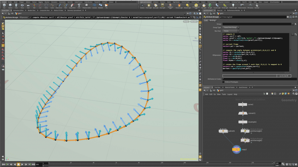
If we want to compute the corresponding quaternionic frame we can do this by applying an appropriate rotation in the normal plane. Therefore one can e.g. wire another point wrangle node which contains the following code:

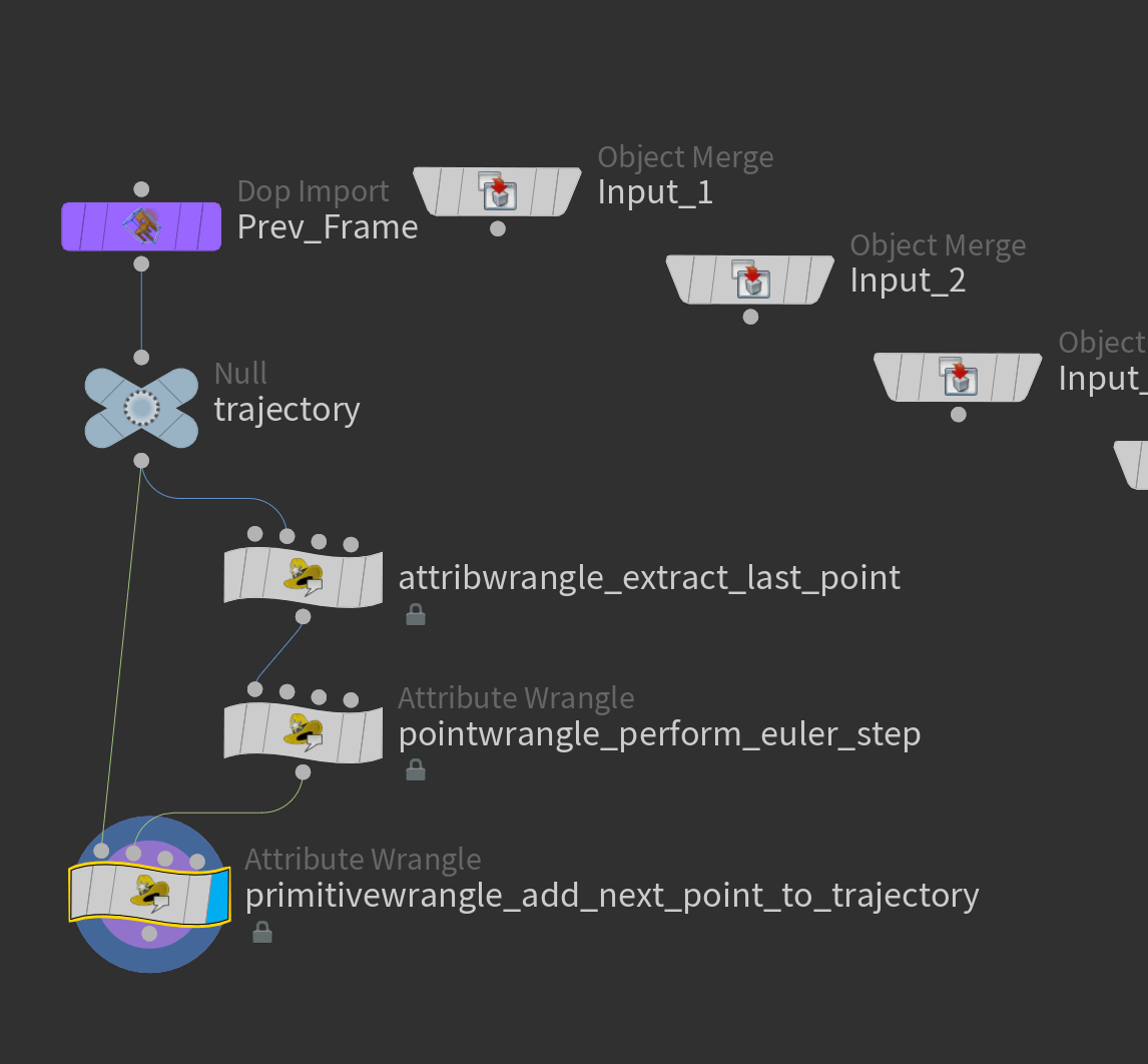
Parallel transport. Let \(\gamma\) be a regular discrete curve. Then, if \(e_{i-1}\times e_i\neq 0\) the parallel transport \(P_i\in\mathrm{SO}(3)\) from edge \(e_{i-1}\) to the edge \(e_i\) is defined to be the unique rotation around \(e_{i-1}\times e_i\) which maps \(T_{i-1}\) to \(T_i\), i.e.\[P_i(e_{i-1}\times e_i) = e_{i-1}\times e_i,\quad P_i(T_{i-1}) = T_i.\]In case that \(e_{i-1}\times e_i =0\) we define \(P_i\) to be the identity. A parallel frame is then a frame \(\sigma\) such that for all \(i\)\[\sigma_i = P_i\sigma_{i-1}.\]So given \(\sigma_0\) we can compute a parallel frame iteratively using the above equation.

This directly translates to the quaternionic setup: Let \(r_i \in \mathbb S^3\subset \mathbb H\) be such that \(P_i(\mathbf v) = r_i\mathbf v\overline{r_i}\). Then a quaternionic frame \(\psi\) is parallel if\[\psi_i = r_i\psi_{i-1}.\]In Houdini it is actually really easy to get the quaternionic parallel transport \(r_i\):\[r_i = \mathtt{dihedral(}T_{i-1},T_i\mathtt{)}.\]We then can compute a parallel frame by an attribute wrangle node (with ‘Run over’ set to ‘detail’) which contains the following code:

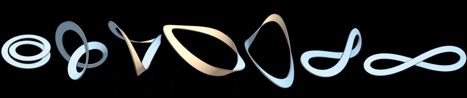
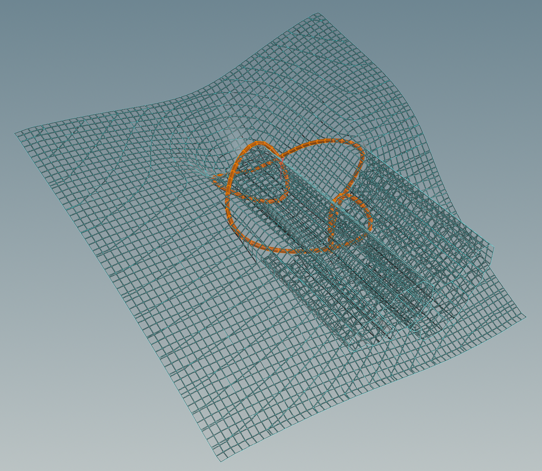
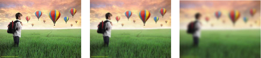
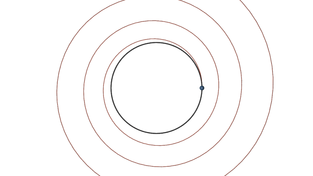
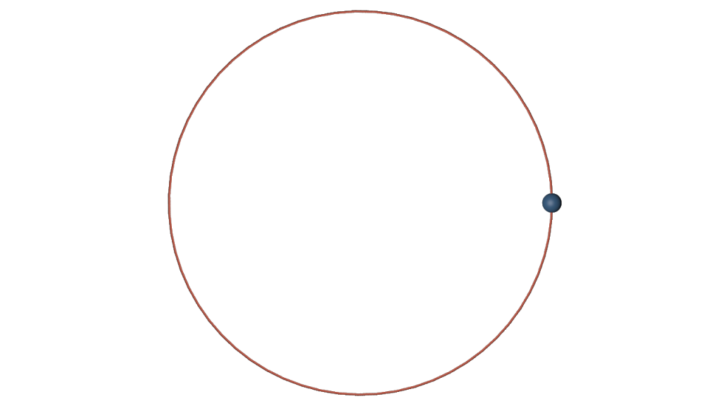
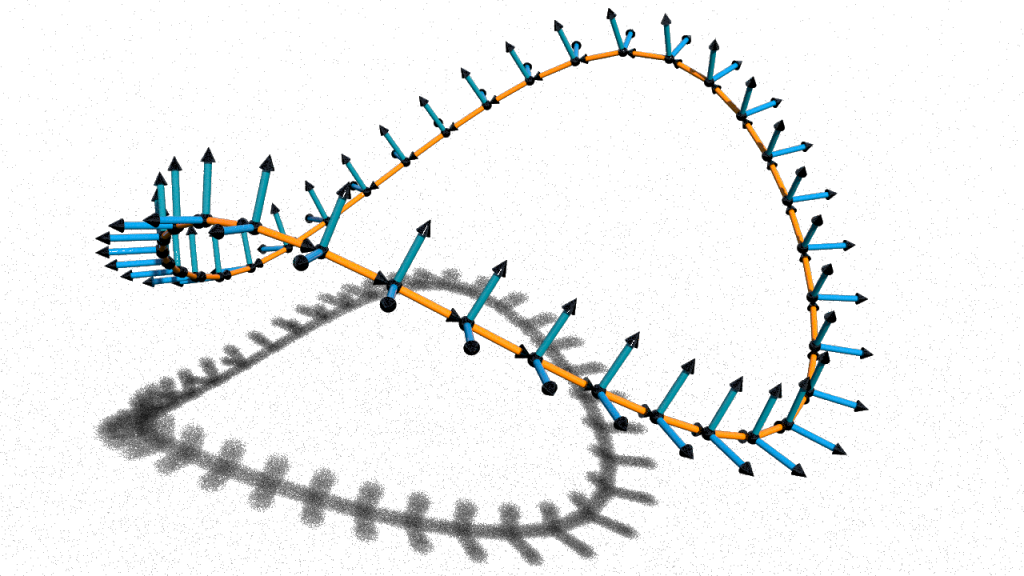
If one applies the algorithm above to a closed curve then the output frame might not close up but return with a phase shift as e.g. shown in the picture below.

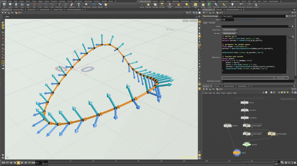
This angle defect is a well-known phenomenon. A closed curve has no global parallel frame in general. If we insist on a global frame, we still can spread the angle defect equally over the edges: Let us assume for simplicity that all edge have equal length. If \(\psi_{n-1}\) is the frame on the last edge, then \(m=\psi_0^{-1}r_{0}\psi_{n-1}\) is a rotation around the \(x\)-axis, i.e. \(m=\cos(\tfrac{\alpha}{2})+ \sin(\tfrac{\alpha}{2})\). If we define\[\tilde\psi_i = \psi_i(\cos(\tfrac{\alpha_i}{2})+\sin(\tfrac{\alpha_i}{2})\mathbf i), \quad \textit{where }\alpha_i = \tfrac{\alpha}{n}i,\]
then \(\tilde\psi\) has a small constant torsion but closes up.

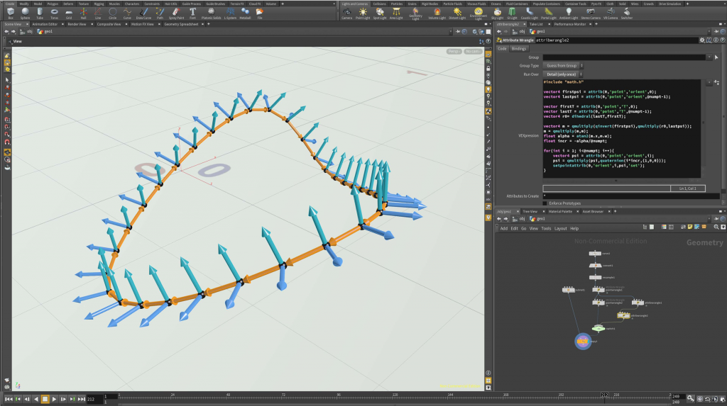
Below the corresponding code of the attribute wrangle node (again ‘Run over’ set to ‘detail’).

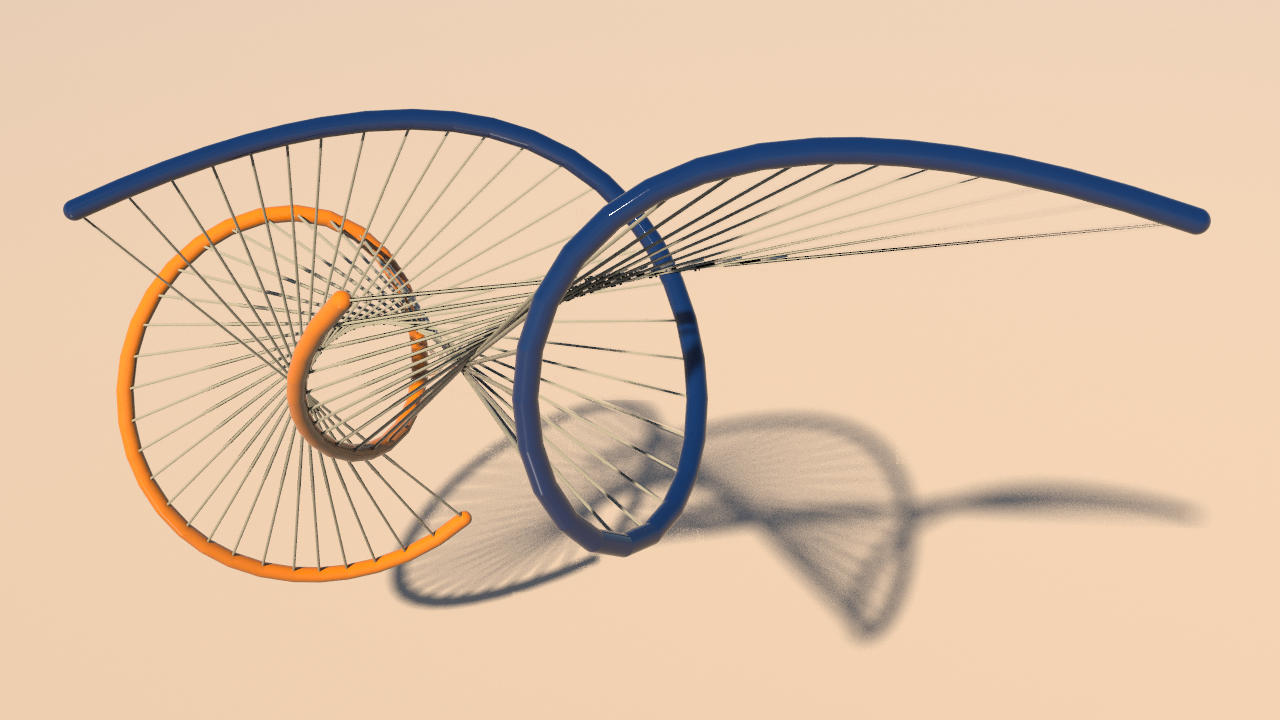
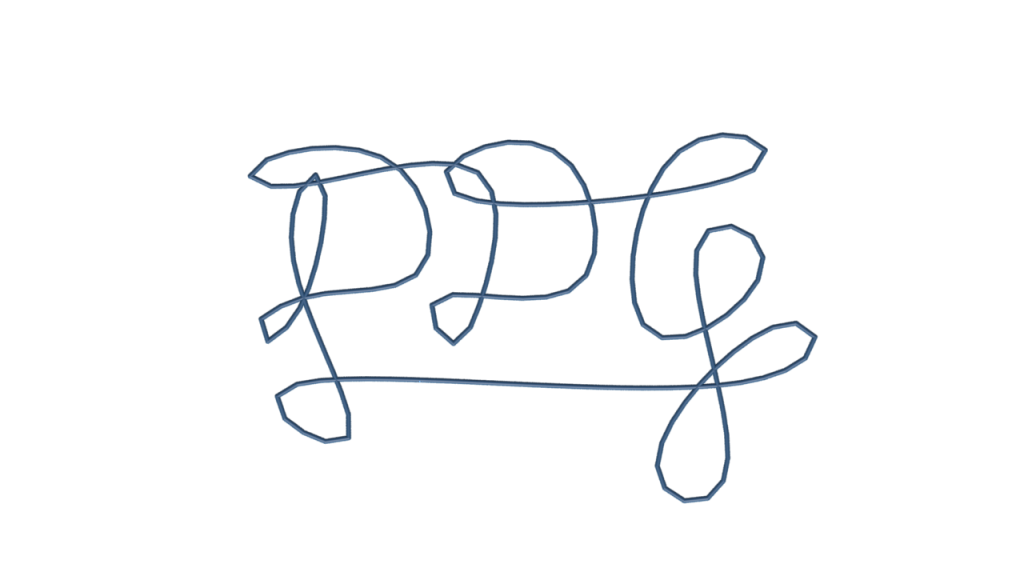
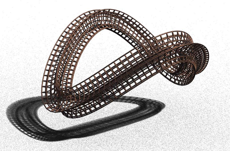
Tubes. Given the framed curve \(\gamma\) it is now easy to draw a tube around it. In principle one can use an arbitrary profile curve \(\eta\). In the picture below we used just a square

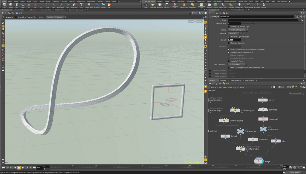
The code is quite easy: We just create a quad meshed torus (torus1) and modify its coordinates by a pointwrangle node which has 3 inputs: the torus (0th input – the geometry we want to modify), the framed curve (1st input) and the profile curve (2nd input). See also the picture above.

int xres = ch('../torus1/cols');
int yres = ch('../torus1/rows');

Homework (due 22 May). Wire up a network that computes for a given profile curve \(\eta\) a tube around a space curve \(\gamma\) as described above.

In this very first tutorial we will describe how to solve initial value problems using Houdini. We will first play this through for an first order ODE – the Lorenz system – before you apply the solver to compute the trajectories of charged particles in a static magnetic field.

Consider a smooth vector field \(f\colon \mathbb R^n\to \mathbb R^n\). We are interested in the solutions \(y\colon \mathbb R \to \mathbb R^n\) of the equation \(y^\prime(t) = f(y(t))\) with \(y(t_0) = y_0\in \mathbb R^n\).

The most naive way to numerically approximate a solution is to successively perform linear steps along the tangent. This leads to the so called Euler method: For a given small time step \(h>0\), we put \[y_{k+1} = y_k + h\,f(y_k).\]

Certainly, we cannot expect high accuracy. E.g., if \(f\colon \mathbb C \to \mathbb C\) is given by \(f(z) = iz\), the exact solutions are circles, while the outcome of the Euler method drifts away from the circle and forms a discrete spiral.

The Euler method is easily implemented using Houdini’s Solver node. Here is how such a network may look like (inside a geometry node):

The Attribute Wrangle node “init trajectory” just takes the initial point (center of a sphere primitive) and turns it in an open polygon (polyline):

The Euler step is performed inside a solver node. Let us dive into the solver node:

Here we use an Attribute Wrangle node (which ‘runs over’ detail) to extract the last point of the trajectory curve,

perform an Euler step (Point Wrangle node).

and add this point to the trajectory curve (Primitive Wrangle node)

A more sophisticated method to solve differential equations is the so called Runge-Kutta method (RK4) It basically consists of 4 Euler steps and schematically this looks as follows:

The scheme translates one to one into a Houdini network which then replaces the single Euler step node of the previous network:

Moreover, we used here a null node to store the step size as a float parameter \(h\). The code of the single nodes is very simple: The pointwrangle_marchhalf1 contains e.g. just 3 lines

Similarly the ‘compute f’ nodes even consist of just one line

With the RK4 method we then obtain for \(h=.1\) a nice circle:

Let us apply this to the Lorenz attractor. We only have to change \(f\). We do this by creating a String parameter ‘code’ (multiline, VEX) in the parameters node.

The code written there then can be imported in wrangle nodes by inserting <code>chs("../parameters/code") at the start of the ‘VEXpression’ field. E.g.

Here how the result then may look like:

The motion of a particle of charge \(q\) in a magnetic field \(B\colon \mathbb R^3 \to \mathbb R^3\) is given by a solution \(\gamma\colon \mathbb R \to \mathbb R^3\) of the second order ODE\[\gamma^{\prime\prime}(t) = q\,\gamma^\prime(t)\times B(\gamma(t)).\]Details can be found various internet pages and articles, as e.g. the Wikipedia article on Lorentz force or this article on the motion in constant and uniform fields.

Homework (due 8 May). Modify the network such that it computes the trajectory of a charged particle moving in the field of a magnetic dipole. Therefore change the RK4 solver such that it operates on a float[] point attribute \(y\) (instead of the point positions), reduce the second order ODE to a first order ODE (on \(\mathbb R^6\)) and solve it.

Further one can use a Scatter node to generate particles equally distributed on a given geometry. Here a picture of 500 particles (with constant initial velocity) shot at a magnetic dipole.