Tutorial 2 – Frames and tubes

Under a discrete space curve \(\gamma\) we understand a (finite or periodic) sequence \(\gamma_i\) of points in \(\mathbb R^3\). The \(i\)-th edge vector is then denoted by \(e_i = \gamma_{i+1} – \gamma_i\) and has length \(\ell_i = |e_i|\). If \(\ell_i\neq 0 \) for all \(i\) we call \(\gamma\) regular and define the tangent vector \(T_i=e_i/\ell_i\).

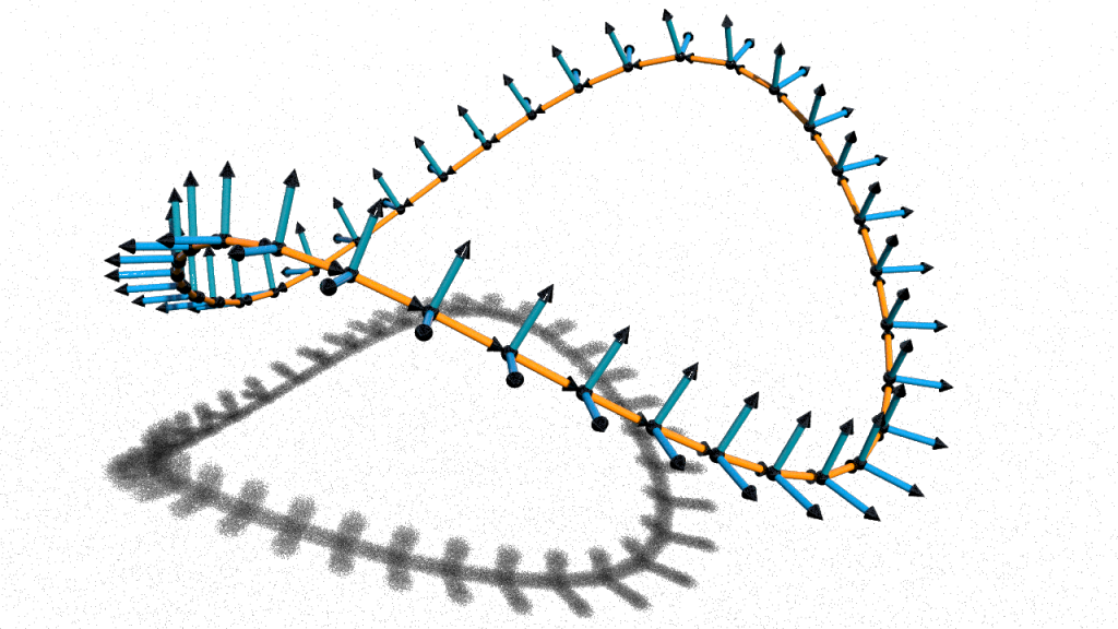
A frame for \(\gamma\) is then an assignment of a positively oriented orthonormal basis \(T_i,N_i,B_i\) to each edge \(e_i\) of \(\gamma\), i.e. to each edge it assigns a rotation \[\sigma_i = (T_i,N_i,B_i) \in \mathrm{SO}(3).\]

Quaternions. The quaternions, denoted \(\mathbb H\), are a number system similar to the complex numbers but with \(3\) linearly independent imaginary units \(\mathbf i, \mathbf j,\mathbf k\): A quaternion \(q \in \mathbb H\) is a number of the form\[q = w + x\,\mathbf i + y\,\mathbf j + z\,\mathbf k, \quad w,x,y,z\in \mathbb R.\]In analogy to the complex numbers we define \(\mathrm{Re}(q) := w\) (real part of \(q\)), \(\mathrm{Im}(q) := x\mathbf i + y\mathbf j + z\mathbf k\) (imaginary part of \(q\)) and \(\bar q = \mathrm{Re}(q)-\mathrm{Im}(q)\) (conjugate of \(q\)).

The quaternionic multiplication is determined by the following multiplication rules:\[\mathbf i^2 = \mathbf j^2 = \mathbf k^2 = -1, \quad \mathbf{i\,j}=\mathbf{k}= -\mathbf{j\,i},\quad \mathbf{j\,k}=\mathbf{i}=-\mathbf{k\,j},\quad \mathbf{k\,i}=\mathbf{j}=-\mathbf{i\,k}.\]

In Houdini the quaternionic multiplication is implemented by the VEX function

• vector4 qmultiply(vector4 q1, vector4 q2)

As quaternions provide a convenient way to represent rotations, they are well-known in Computer Graphics. In Houdini they appear as \(4\)-vectors:\[\mathbb R^4 \ni \mathbf (w,x,y,z) \longleftrightarrow w + x\,\mathbf i + y\,\mathbf j + z\,\mathbf k \in \mathbb H.\]So what has this to do with rotations in Euclidean \(3\)-space? Let us identify \(\mathbb R^3\) with the purely imaginary quaternions \(\mathrm{Im}\, \mathbb H = \mathrm{span}_{\mathbb R}\{\mathbf i,\mathbf j,\mathbf k\}\)\[\mathbb R^3 \ni \mathbf (x,y,z) \longleftrightarrow x\,\mathbf i + y\,\mathbf j + z\,\mathbf k \in \mathrm{Im}\,\mathbb H.\]Let \(q = \cos(\tfrac{\alpha}{2}) + \sin(\tfrac{\alpha}{2})\mathbf a\) with \(\alpha \in \mathbb R\) and \(\mathbf a \in \mathbb S^2 \subset \mathrm{Im}\,\mathbb H\), then the map \(R_q\colon \mathbb R^3 \to \mathbb R^3\) given by\[\mathbf v \mapsto q\mathbf v \bar q\]is a (positive) rotation by the angle \(\alpha\) around the vector \(\mathbf a\). If one is used to quaternionic algebra this is easy to see. We skip this here. A proof can be found e.g. in the DDG 2016 blog.

The maps \((\alpha,\mathbf v)\mapsto \cos(\tfrac{\alpha}{2}) + \sin(\tfrac{\alpha}{2})\mathbf v\) and \((q,\mathbf v) \mapsto R_q(\mathbf v)\) are built into Houdini by the following VEX functions:

• vector4 quaternion(float angle, vector axis)
• vector qrotate(vector4 quaternion, vector a)

Remark. It is an easy exercise to check that \(\overline{q_1q_2} = \overline{q_2}\,\overline{q_1}\). Thus \(\mathbb S^3 = \{q\in\mathbb H \mid |q|^2 = \bar q q = 1\}\) forms a group. Moreover, \(R_{q_1}\circ R_{q_2} = R_{q_1q_2}\), i.e. the map \(\mathbb S^3 \to \mathrm{SO}(3)\), \(q\mapsto R_q\) is a group homomorphism. Actually it is a \(2\)-sheeted covering, \(R_{q} = R_{-q}\).

Quaternionic frames and the Copy Stamp node. Let \(\gamma\) be a regular discrete space curve. A discrete frame is a map which assigns to each edge \(e_i\) of \(\gamma\) a rotation \(\sigma_i \in \mathrm{SO}(3)\) such that\[T_i = \sigma_i\left(\begin{smallmatrix}1\\0\\0\end{smallmatrix}\right),\quad N_i = \sigma_i\left(\begin{smallmatrix}0\\1\\0\end{smallmatrix}\right), \quad B_i = \sigma_i\left(\begin{smallmatrix}0\\0\\1\end{smallmatrix}\right)\]A quaternionic frame \(\psi\) is then a lift of \(\sigma\), i.e. for all \(i\) we have \(\psi_i\in\mathbb S^3\) such that \(\sigma_i = R_{\psi_i}\). In particular, we have\[T_i = \psi_i\,\mathbf i\,\bar{\psi_i}, \quad N_i = \psi_i\,\mathbf j\,\bar{\psi_i}, \quad B_i = \psi_i\,\mathbf k\,\bar{\psi_i}.\]For the visualization we can use Houdini’s Copy Stamp node. Looking at its Copying and instancing point attributes we find that this node can handle quaternionic frames out of the box (there appearing as the point attribute @orient). Moreover we can specify for each point a scale factor (point attribute @pscale).

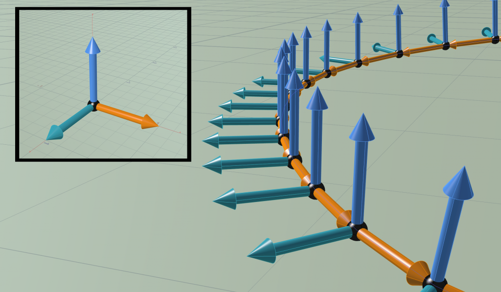
The picture below shows how such a network could look like.

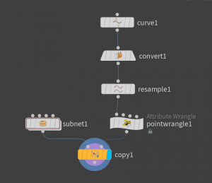
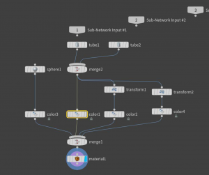
The subnet1 node merges colored tubes and a sphere to visualize the standard frame. The network is shown in the picture below.

So far the VEX code contained in pointwrangle1 produces just some arbitrary frame:

The method dihedral(vector a, vector b) returns a quaternion which represents a rotation around the vector \(a\times b\) which takes the vector \(a\) to the vector \(b\).

Frénet frame. Let us assume that we are dealing with a discrete Frénet curve, i.e. \(e_i\times e_{i+1}\neq 0\). Then this defines a frame \((T_i,N_i,B_i)\) by\[B_i = T_i\times N_i\quad with \quad B_i = \frac{e_i\times e_{i+1}}{|e_i\times e_{i+1}|}.\]

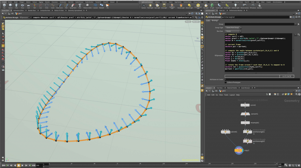
If we want to compute the corresponding quaternionic frame we can do this by applying an appropriate rotation in the normal plane. Therefore one can e.g. wire another point wrangle node which contains the following code:

Parallel transport. Let \(\gamma\) be a regular discrete curve. Then, if \(e_{i-1}\times e_i\neq 0\) the parallel transport \(P_i\in\mathrm{SO}(3)\) from edge \(e_{i-1}\) to the edge \(e_i\) is defined to be the unique rotation around \(e_{i-1}\times e_i\) which maps \(T_{i-1}\) to \(T_i\), i.e.\[P_i(e_{i-1}\times e_i) = e_{i-1}\times e_i,\quad P_i(T_{i-1}) = T_i.\]In case that \(e_{i-1}\times e_i =0\) we define \(P_i\) to be the identity. A parallel frame is then a frame \(\sigma\) such that for all \(i\)\[\sigma_i = P_i\sigma_{i-1}.\]So given \(\sigma_0\) we can compute a parallel frame iteratively using the above equation.

This directly translates to the quaternionic setup: Let \(r_i \in \mathbb S^3\subset \mathbb H\) be such that \(P_i(\mathbf v) = r_i\mathbf v\overline{r_i}\). Then a quaternionic frame \(\psi\) is parallel if\[\psi_i = r_i\psi_{i-1}.\]In Houdini it is actually really easy to get the quaternionic parallel transport \(r_i\):\[r_i = \mathtt{dihedral(}T_{i-1},T_i\mathtt{)}.\]We then can compute a parallel frame by an attribute wrangle node (with ‘Run over’ set to ‘detail’) which contains the following code:

If one applies the algorithm above to a closed curve then the output frame might not close up but return with a phase shift as e.g. shown in the picture below.

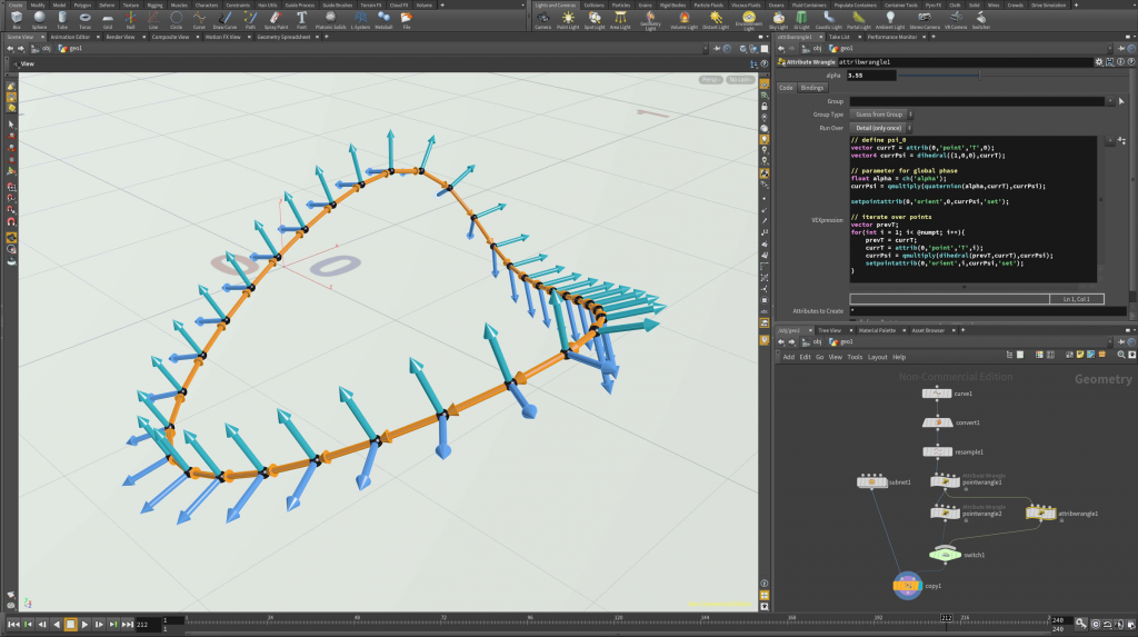
This angle defect is a well-known phenomenon. A closed curve has no global parallel frame in general. If we insist on a global frame, we still can spread the angle defect equally over the edges: Let us assume for simplicity that all edge have equal length. If \(\psi_{n-1}\) is the frame on the last edge, then \(m=\psi_0^{-1}r_{0}\psi_{n-1}\) is a rotation around the \(x\)-axis, i.e. \(m=\cos(\tfrac{\alpha}{2})+ \sin(\tfrac{\alpha}{2})\). If we define\[\tilde\psi_i = \psi_i(\cos(\tfrac{\alpha_i}{2})+\sin(\tfrac{\alpha_i}{2})\mathbf i), \quad \textit{where }\alpha_i = \tfrac{\alpha}{n}i,\]
then \(\tilde\psi\) has a small constant torsion but closes up.

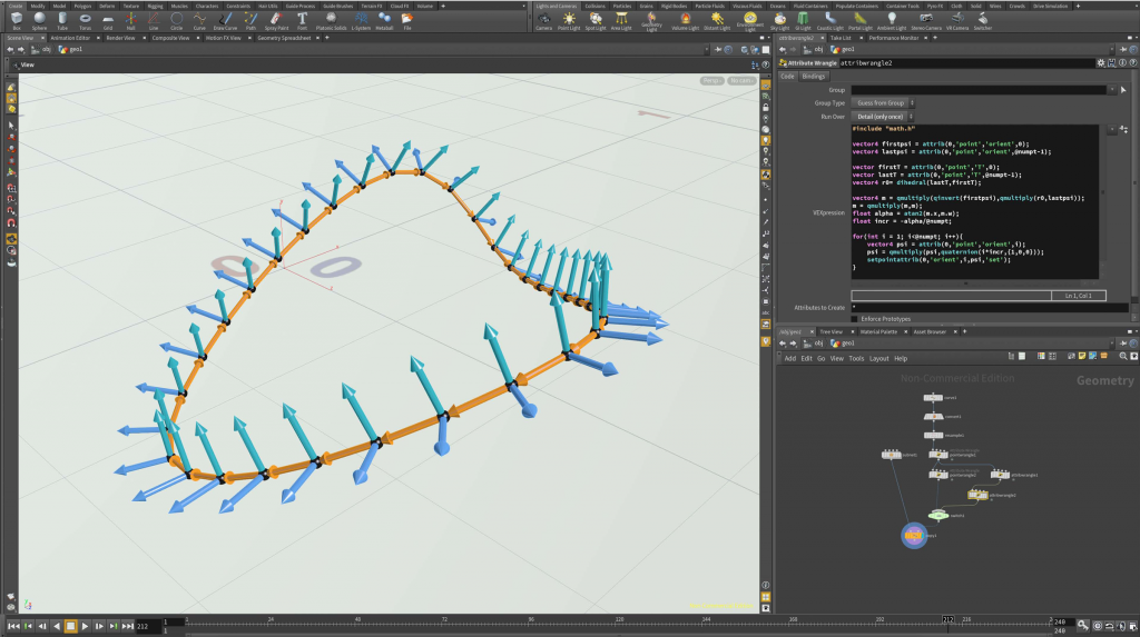
Below the corresponding code of the attribute wrangle node (again ‘Run over’ set to ‘detail’).

Tubes. Given the framed curve \(\gamma\) it is now easy to draw a tube around it. In principle one can use an arbitrary profile curve \(\eta\). In the picture below we used just a square

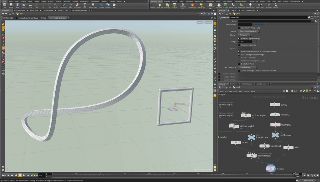
The code is quite easy: We just create a quad meshed torus (torus1) and modify its coordinates by a pointwrangle node which has 3 inputs: the torus (0th input – the geometry we want to modify), the framed curve (1st input) and the profile curve (2nd input). See also the picture above.

int xres = ch('../torus1/cols');
int yres = ch('../torus1/rows');

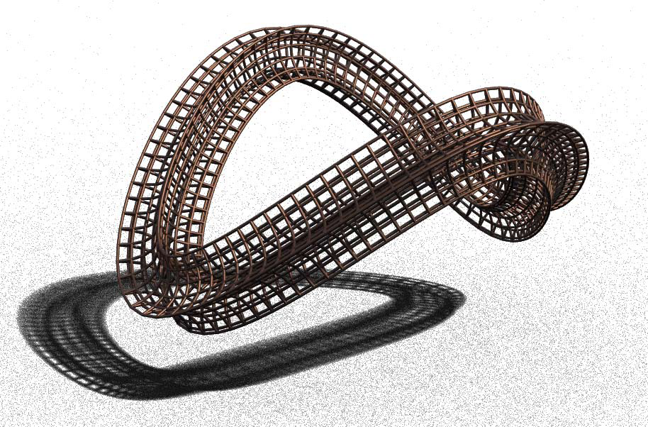
Homework (due 22 May). Wire up a network that computes for a given profile curve \(\eta\) a tube around a space curve \(\gamma\) as described above.