
The goal of this post is to implement certain time-continuous flows on discrete space curves. By a time-continuous flow of a closed discrete space curve \(\gamma\colon \mathbb Z/n\mathbb Z \to \mathbb R^3\) we mean the continuous solution of an equation\[\dot\gamma = X(\gamma)\]Here \(X\) is vector field on the space of discrete curves, i.e. a map that assigns to a curve \(\gamma\) with \(n\) vertices a sequence \(X(\gamma)\colon \mathbb Z/n\mathbb Z \to \mathbb R^3\).
In this post we will focus on the Möbius tangent flow, which is a discrete analogue of the continuous tangent flow \(\dot\gamma = \gamma^\prime\), and a discrete analogue of the continuous vortex filament flow \(\dot\gamma = \gamma^\prime \times \gamma^{\prime\prime}\). Here \((.)^\prime\) denotes the derivative with respect to arclength.
While in the continuous setup the tangent flow is trivial (it just acts by reparametrization), the discrete tangent flow will change the shape of the polygon.
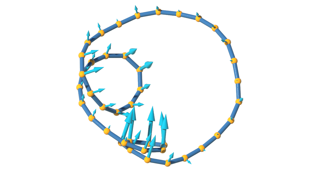
Given a closed discrete space curve with \(n\) vertices, i.e. \(\gamma\colon \mathbb Z/n\mathbb Z \to \mathbb R^3\), then for each edge we have an edge vector \[S_i = \gamma_{i+1}-\gamma_i\]This provides a canonical (unit) tangent vector along each edge. Though at a vertex itself there is no obvious choice of a tangent vector – there is a whole interval of candidates.
E.g. one reasonable choice for \(T_i\) could be the angle bisector between \(S_{i-1}\) and \(S_i\), i.e. \[\Bigl(\tfrac{S_{i-1}}{|S_{i-1}|}+\tfrac{S_i}{|S_i|}\Bigr)/\Bigl|\tfrac{S_{i-1}}{|S_{i-1}|}+\tfrac{S_i}{|S_i|}\Bigr|\]Another possible definition of \(T\), leading to a much more stable and, in fact, Möbius invariant flow is given by the harmonic mean of \(S_{i-1}\) and \(S_i\), i.e.\[T_i=\frac{|S_{i}|^2S_{i-1} + |S_{i-1}|^2S_i}{|S_{i-1}+S_i|^2}\]Note that for arc length parametrized \(\gamma\), i.e. \(|S_i| = 1\), both definitions coincide. Details can be found e.g. in Tim Hoffmann’s lecture on Discrete Differential Geometry of Curves and Surfaces or Alexander Bobenko’s script on Discrete Differential Geometry.
Mainly the flow \(\dot\gamma = T\) just shifts the vertices along the curve. Though if we run the simulation at high speed the shape of the curve changes essentially, as shown in the following video.
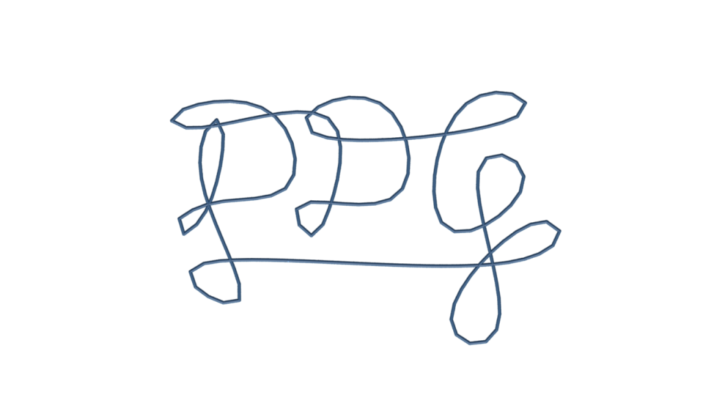
We observe loops traveling along the curve, interacting when passing each other while basically keeping their shape. This kind of phenomenon hints at a connection to soliton theory.
Another flow related to soliton theory is the vortex filament flow. It describes how vortex filaments move and is related to the cubic non-linear Schrödinger equation – an equation well-known to soliton theorists.
To motivate the discrete vortex filament flow let us look at the continuous equation and assume for a second that we are dealing with a Frenet curve, i.e. \(\gamma^{\prime\prime} \neq 0\). Here again \((.)^\prime\) denotes the derivative with respect to arc length. Then with \(T= \gamma^\prime\), \(N = \gamma^{\prime\prime}/|\gamma^{\prime\prime}|\) and \(B =T\times N\) we get \(\gamma^{\prime\prime}= \kappa N\) and the vortex filament flow becomes\[\dot\gamma = \kappa B\]The function \(\kappa\) is the so called Frenet curvature of \(\gamma\) and equals the the inverse radius of the osculating circle.
Certainly a discrete curve is not a Frenet curve. Though unless \(S_{i-1}\) and \(S_i\) are parallel there is an osculating plane and a corresponding normal \(B_i\) perpendicular to that plane which was already used in a previous post to define the discrete Frenet frame. But what is a discrete Frenet curvature? Again there is no canonical choice and several choices are presented in the scripts mentioned above. We will just stick here to the definition using vertex osculating circles as in Tim Hoffmann’s paper, i.e.\[\kappa_i = \frac{2\sin(\alpha_i)}{|S_{i-1}+S_i|}\]where \(\alpha_i\) denotes the angle between \(S_{i-1}\) and \(S_i\). Thus we get\[k_iB_i = \frac{2\,S_{i-1}\times S_i}{|S_{i-1}||S_{i-1}+S_{i}||S_i|}\]
The surface swept out by the vortex filament flow are called Hashimoto surfaces. They can be easily visualized with help of Houdini’s trail node. The point attribute @Alpha controls the alpha channel of the point color and can be used to fade out the trail. Here is a picture how such a surface can look like.
![]()
Homework (due 29 May). Use your Runge-Kutta solver to compute the Möbius tangent and vortex filament flow of a prescribed closed discrete space curve.
Update: Albert has written a digital asset which makes it possible to plot how certain quantities (stored as detail attribute) evolve under the flow.
Homework (due 5 June). Plot the length, the area (projected to a plane) and the energy of a curve (with constant edge length) moving under the tangent and the vortex filament flow. Here energy is defined by \(E = \frac{2}{\ell}\sum_{i}\log(1+\tan^2(\frac{\alpha_i}{2}))\), where \(\ell\) denotes the edge length.