
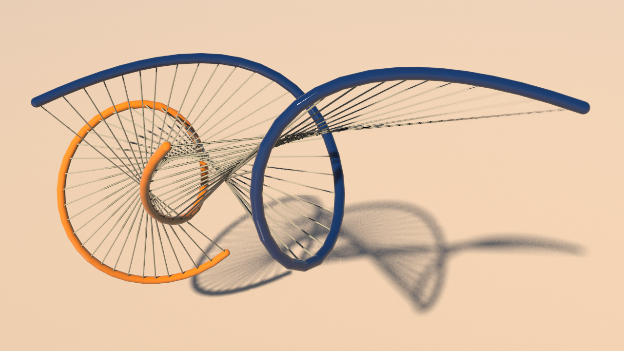
In class you defined the Darboux transformation \(\eta\colon \mathbb R\to \mathbb R^3\) of a smooth space curve \(\gamma\colon \mathbb R\to \mathbb R^3\). By construction, the distance between corresponding points is constant. Or phrased differently, there is \(S\colon \mathbb R \to \mathbb S^2 \subset \mathbb R^3\) such that \[\eta=\gamma + \ell S.\]Moreover, you proved that Darboux transformations preserve arc length. This led to the following definition of the discrete Darboux transformation: A discrete space curve \(\eta\colon \mathbb Z \to \mathbb R^3\) is called a Darboux transformation of a discrete space curve \(\gamma\colon \mathbb Z \to \mathbb R^3\) with rod length \(\ell\) and twist \(r\) if \[\eta_j = \gamma_j + \ell S_j,\] where \(S\colon \mathbb Z \to \mathbb S^2\) satisfies\[S_{j+1} =(r+\ell S_j-v_jT_j)S_j(r+\ell S_j-v_jT_j)^{-1}.\]Here \(v_jT_j = \gamma_{j+1}-\gamma_j\) with \(v_j=|\gamma_{j+1}-\gamma_j|\). Compare also with this post from 2013.
The discrete Darboux transformation is easily implemented – given a discrete space curve \(\gamma=(\gamma_0,\ldots,\gamma_{n-1})\), a point \(p\in\mathbb R^3\) and \(r\in \mathbb R\), then we obtain a discrete Darboux transformation \(\eta\) of rod length \(\ell := |\gamma_0 – p|\) and twist \(r\) starting at \(p\) (\(\eta_0 = p\)) as follows:
- Set \(S_0 := (\eta_0 – \gamma_0)/\ell\),
- iteratively compute \(S\), and
- define \(\eta_j := \gamma_j + \ell S_j\).
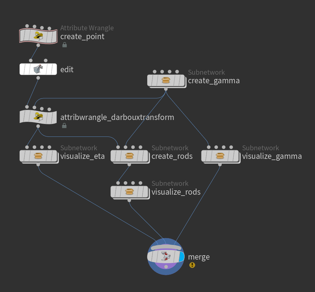
As we want to play around with the Darboux transformation we want to have control over the initial data \(p\) and \(r\). The parameter \(r\) can be just given as a node parameter. The initial point \(p\) can just be given by a geometry containing just a single point which is then made draggable by an edit node. Here is how such a network could look like:
In general, a Darboux transformation of a closed discrete space curve \(\gamma \colon \mathbb Z/n\mathbb Z \to \mathbb R^3\) is not closed. Though, for given \(\ell\) and \(r\) the map \(M_{\ell,r} \colon \mathbb R^3 \to \mathbb R^3\) sending the initial rod direction \(S_0\) to the end rod direction \(S_n\) is a Moebius transformation, a generic discrete space curve will have exactly two closed Darboux transformations corresponding to the fixed points of \(M_{\ell,r}\). These points could be computed directly from \(M_{\ell,r}\). Unfortunately if we try to compute \(M_{\ell,r}\) we run into numerical problems . Fortunately, we quickly converge to a fixed point when running around \(\gamma\) several times (always computing a new Darboux transformation starting from the end of the previous).

Affectively this amounts to applying \(M_{\ell,r}\) several times but turns out to be numerically stable and quite fast. So we can compute a closed Darboux transformation of a discrete space curve \(\gamma\colon \mathbb Z/n\mathbb Z \to \mathbb R^3\) with rod length \(\ell\) and twist \(r\) as follows:
- Compute for sufficiently large \(m \in\mathbb N\) the direction \(\tilde S_{mn}\) starting from some initial rod direction \(S_0\in\mathbb S^2\),
- Compute the Darboux transformation \(\eta\) starting at \(\gamma_0+\ell \tilde S_{mn}\).
Similarly, a second fixed point is found when running \(\gamma\) backwards (iterating \(M_{\ell,r}^{-1}\)).
![]()
Homework (due 19 June). Write a digital asset which computes for a closed discrete space curve a closed Darboux transformation with rod length \(\ell\) and twist \(r\). Use a checkbox to specify whether to iterate forward of backward.