In your next homework, you will have to deal with conformal mappings. To do this, there are a few things we still have to learn.


But first a note on assets.
Assets
How do you reuse code in Houdin? If you don’t value your time in this life you could always copy and paste your nodes. A faster approach is to create your own digital assets.
Creating a digital asset is like creating a node of your own. This new node will consist of a collection of sub-nodes and can have exchangeable parameters of its own.
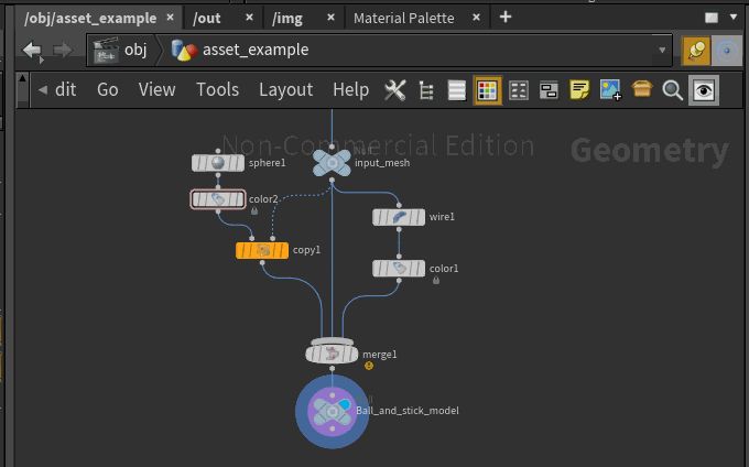
To create an asset you first have to set up a couple of nodes that create the function that defines your asset. For example, you might want to reuse this simple ball and stick model network

To create a digital asset from these nodes, highlight them all and create a subnetwork
Now you can right-click on this subnet and “create digital asset“
You can now store your digital asset in a .hda (.hdanc for non-comercial) file. One such file can contain multiple assets.

That is it! You can now drop a ball and stick node wherever you like

To import digital assets in your next project click on assets->install asset library

Editing Assets
Notice the cute little lock when using assets. It remains locked when the assets not being edited. Right-click on the node to unlock it by “allow editing of content”


Then you can change whatever you want locally. However, in order to save the changes onto the asset and thus update all instances of this assets you must right-click and select Save Node Type.

If instead, you click on Match Current Definition you will reset your edits to the current .hda version.
Building Parameters
Let’s say that your ball and stick method needs a handle to edit the size of the spheres. To expose an editable parameter simply right click on the node after unlocking it and hit Type Properties.

Here you can create and edit parameters to be exposed in the interface and even edit the icon of your node.

Once you have created a float parameter that you call sphere_size you can now edit it when clicking on the node.

Right-clicking on the node will allow you to copy the parameter. This is extremely useful because now you can paste the reference to the parameter where the size of your sphere is determined. Use paste relative references to be functional in other files as well.


It will now say ch(“../sphere_size”) in the place where you have pasted it. Now don’t forget to save your asset again. Now you can slide the sphere size with you mouse directly from the asset:

Your Homework 06 will make use of this.
Conformal Mappings
We are merciful and allow you to implement this yourself. The lecture notes 06_Conformal.pdf contain the description of the algorithm that you will be using for your homework.


Lucky for you, we provide you with DEC assets that will reduce your implementation effort. The first node called DEC_build will compute point weights, cotan weights, lengths, areas, label boundaries, source points, and destination points, reference opposite edges and so on. It’s two outputs will be the original mesh as well as the primal edge graph used for matrix building.

The second node, DEC_matrices, builds all your favorite matrices that you love so much. It even allows you to specify the name you want these matrices to have. This asset needs two inputs, which are the two outputs of the DEC_build.

Go ahead and read the notes from 06_Conformal.pdf and implement it yourself as your homework.
Note: In the visualization industry, an “asset” can be any sharable, reusable item. Algorithms, textures, models, sounds, music, materials, environmental lights etc… Online stores can be used to distribute and sell these assets. A robust solid algorithm can be worth a lot online and now you already have the tools to build a user-friendly one.
Notes on Python
Complex numbers
As you might have noticed the algorithm for conformal mappings requires complex numbers in python. Theoretically, you can work well with two float values, which is what you should do on a VEX level. In Python, however, complex numbers can be defined directly.
Look how easy python works with complex numbers. Just work with j
z = 2 + 3j
w = 0.5 + 0.1j
print z*w
( this will print 0.7+1.7j )
This is how you create an array of complex numbers of size n
w = np.zeros( n , dtype=np.complex_)
This is how you can get the real and imaginary parts from an array
np.real( … ), np.imag( … )
SciPy methods
scipy.sparse.linalg has eigenvalue and eigenvector methods also for the generalized eigenvalue problem. You can also Cholesky factorization and use the inverse power method.
Hint on Houdini and Python
By default, you have seen node = hou.pwd(). pwd is the present working directory and this call gives you a handle to your node. Then geo = node.geometry() creates a handle to access the geometry of the node.
You can input the edge skeleton (primal graph) as your second input. In python you can then access the second input using node_edge = node.inputs()[1]. Using this handle you can access geo_edge = node_edge.geometry() and now read attributes from the second input into python.

Using such a geometry node handle also allows you to iterate over all elements of a node. For example:
for prim in geo_edge.prims():
# will iterate over every primitive of the node geo_edge
Now you are ready for the homework!
