Projective Geometry

Let us start with a general definition for an arbitrary projective space. In this lecture we will almost entirely deal with real projective spaces.

Definition. Let $V$ be a vector space over an arbitrary field $F$. The projective space $P(V)$ is the set of $1$-dimensional vector subspaces of $V$. If $\dim(V) = n+1$, then the dimension of the projective space is $n$.

• A $1$-dimensional projective space is a projective line.
• A $2$-dimensional projective space is a projective plane.

Canonical analytic description

Two vectors $v$ and $\tilde{v}$ span the same $1$-dimensional subspace if there exist $\lambda \neq 0$ such that $v = \lambda \tilde{v}$. This yields an equivalence relation on $V \setminus \{0\}$:
\[ v \sim \tilde{v}
:\Leftrightarrow \exists \lambda\neq0 : v = \lambda \tilde{v}.
\]
The points of the projective space $P(V)$ are equivalence classes of $\sim$:

\[P(V) = (V \setminus \{0\})/{\sim}.\]

We write $[v] \in P(V)$ and call $v$ a representative vector of the line $\{\lambda v \,|\, \lambda \in F\}$.

Models of real projective space

Let us have a look at different models for real projective space $\RP^2 = P(\R^3)$.

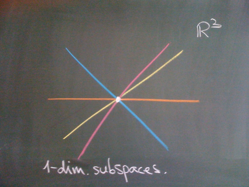
Subspace model

Consider all $1$-dimensional subspaces $\ell = \{\lambda v \,|\, v \in \R^3, v \neq 0, \lambda \in \R\}$ of $\R^n$.

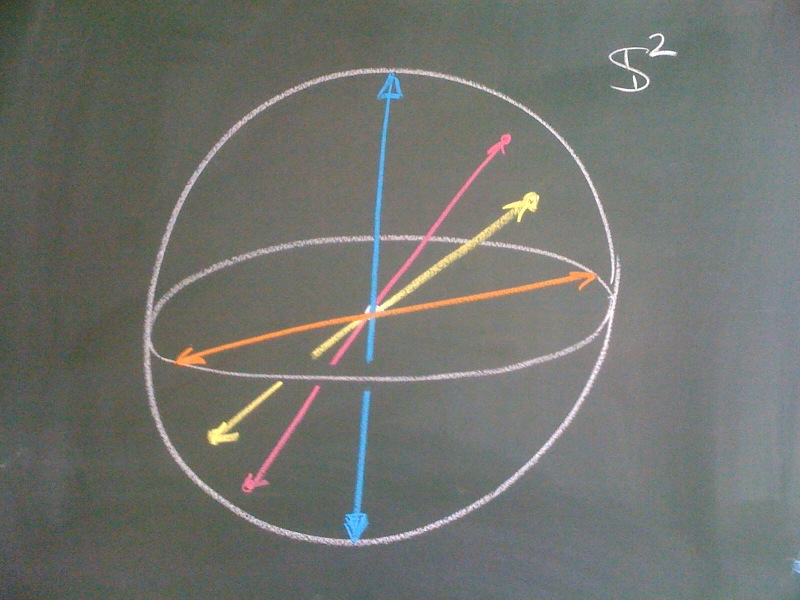
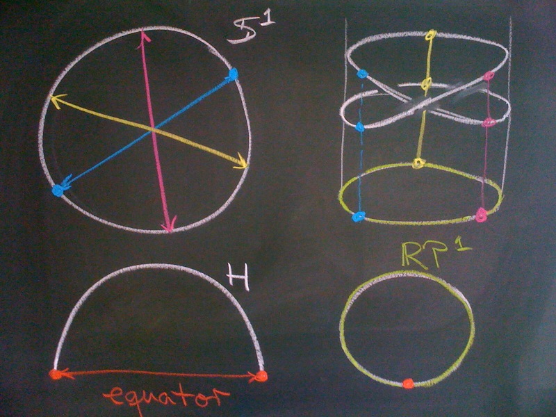
Sphere model

We may normalize non-zero vectors to become unit vectors. Then there are only two vectors representing the same line. If we now introduce an equivalence relation

\[
v \sim \tilde{v} \quad :\Leftrightarrow \quad
v = \pm\tilde{v} \text{ for $v,\tilde{v} \in \S^n$}
\]

we obtain $\RP^n = \S^n/\sim$.

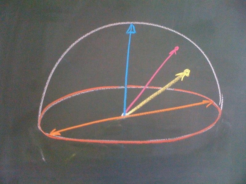
Hemisphere model

Consider the upper hemisphere $H = \left\{ \svector{x_1\\x_2\\x_3} \in \R^3 \,|\, \|x\| = 1, x_3 \geq 0 \right\}$. Then all non-horizontal lines have a unique representative vector in $H$ and we only need to identify points on the equator $H \cap \{ x \,|\, x_3 = 0 \}$.

Examples of lower dimension:

• $\RP^0 = P(\R^1) = \S^0{/}{\sim} = \{*\}$ is just a single point.
• $\RP^1 = P(\R^2) = \S^1{/}{\sim} = \S^1$. This is most obvious using the hemisphere model, since the hemisphere is just a line and the two points on the equator are identified (bottom of the picture below). But we can also twist an $\S^1$ in a way such that opposite points come to lie on top of each other (top of picture below).

Homogeneous coordinates

Consider a basis $\{b_1, \ldots,b_{n+1}\}$ of the vector space $V$ and a vector $v\in V$, $v \neq 0$ with coordinates $(x_1,\ldots,x_{n+1})$, i.e. $v = \sum_{i=0}^{n+1} x_i b_i$. Then $(x_1,\ldots,x_{n+1})$ are homogeneous coordinates of $[v] \in P(V)$. These coordinates are not unique. They depend on the choice of basis and are then only unique up to a scalar factor:
\[
[v] = [x_1,\ldots,x_{n+1}] = [\lambda x_1, \ldots, \lambda x_{n+1}]
\text{, for $\lambda\neq 0$}.
\]

Homogeneous coordinates of $\RP^n$. Let $[v] \in \RP^n$ with coordinates $[v] = [x_1,\ldots,x_{n+1}]$. Since the homogeneous coordinates are only unique up to a scalar factor we do the following:

• if $x_{n+1} \neq 0$ then
  \[[v] = [x_1,\ldots,x_{n+1}]=\left[\frac{x_1}{x_{n+1}},\ldots,\frac{x_n}{x_{n+1}},1\right]=[y_1,\ldots,y_{n+1}] \simeq\R^n.\]
  The coordinates $(y_1,\ldots,y_{n+1})$ are affine coordinates for $[v]$ with $x_{n+1} \neq 0$.
• if $x_{n+1} = 0$ then
  \[ [v] = [x_1,\ldots,x_n,0] \simeq \RP^{n-1}.\]

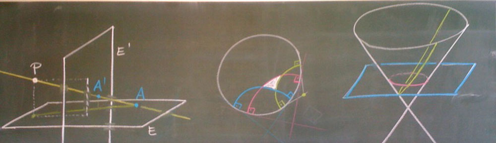
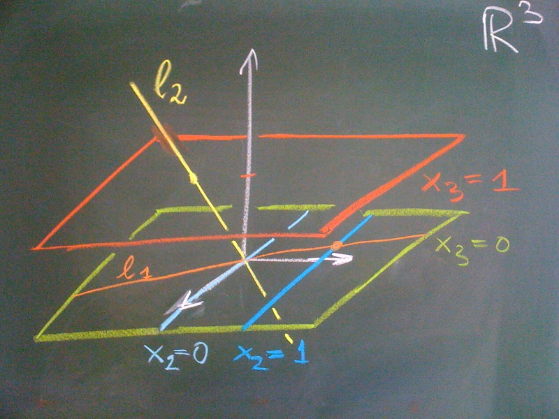
So we obtain the following decomposition $\RP^n = \R^n \cup \RP^{n-1}$. This can be iterated and $\RP^{n-1}$ may again be decomposed into $\R^{n-1}$ and $\RP^{n-2}$, and so on. The part isomorphic to $\R^n$ (e.g. $x_{n+1} \neq 0$) is called the affine part of $\RP^n$ and the other part isomorphic to $\RP^{n-1}$ (e.g. $x_{n+1} = 0$) is called the part at infinity. So in case of $\RP^1$ we have a point at infinity, in case of $\RP^2$ there is an entire projective line at infinity. The following picture shows the decomposition of $\RP^2$ into parts $\R^2$ (the red $x_3 = 1$ plane) and the line at infinity $\RP^1$ corresponding to the lines in the green $x_3 = 0$ plane. Of course, the $x_3 = 0$ plane may itself be decomposed into an affine part, the dark blue line $x_2 = 1$ (and $x_3 = 0$) and the point at infinity represented by the light blue line $x_2 = 0$ (and $x_3 = 0$).

Remarks.

1. To introduce an affine coordinate on a projective space we may choose an arbitrary linear form $\ell(x)=\sum_{i=1}^{n+1} a_i x_i$ on $V$ and decompose the points of the projective space depending on whether $\ell(x) = 0$ or $\ell(x) \neq 0$. In the decomposition above the linear form is $\ell(x) = x_{n+1}$.
2. A projective space should be thought of as a “homogeneous object” (to be made precise). So there are no preferred directions (points of projective space) as the hemisphere model or the introduction of an affine coordinate might suggest.
3. The same definitions are used in the complex case and yield complex projective spaces: $\CP^1 = \C \cup \{\infty\} = \hat\C$ is the Riemann sphere or complex projective line.

Definition. A projective subspace of the projective space $P(V)$ is a projective space $P(U)$ where $U$ is a vector subspace of $V$. If the dimension of $P(U)$ is $k$ (the corresponding vector subspace has dimension $k+1$), the we call $P(U)$ a $k$-plane.
A $0$-plane is a point, a $1$-plane a line, a $2$-plane a plane, and if $P(V)$ has dimension $n$ a $(n-1)$-plane is a hyperplane.

Proposition 2.1. Through any two distinct points in a projective space there passes a unique projective line.

Proposition 2.2. In a projective plane two distinct projective lines intersect in a unique point.

These two propositions can be proved using linear algebra. Further properties of vector subspaces may be transferred to properties of projective subspaces:

1. The intersection of two projective subspaces $P(U_1)$ and $P(U_2)$ is $P(U_1) \cap P(U_2) = P(U_1 \cap U_2)$.
2. The projective span or join of two projective subspaces $P(U_1)$ and $P(U_2)$ is $P(U_1 + U_2)$.
3. From the dimension formula of linear algebra we obtain a dimension formula for projective subspaces:
   \begin{align*}
   \dim(U_1 + U_2) &= \dim U_1 + \dim U_2 – \dim (U_1 \cap U_2) \\
   \dim P(U_1 + U_2) &= \dim P(U_1) + \dim P(U_2) – \dim P(U_1) \cap P(U_2)
   \end{align*}