Consider the space
$$C^0(\mathbb{Z}^n)= \{f:\mathbb{Z}^n \to \mathbb{R} \,\,|\,\, f\text{ is bounded} \}.$$
Suppose we have a probability distribution $p$ on $\mathbb{Z}^n$ with mean zero:
\begin{align*}p:\mathbb{Z}^n &\to \mathbb{R} \\\\ p(\mathbf{n})&\geq 0 \quad \text{for all}\quad \mathbf{n}\in \mathbb{Z}^n\\\\ \sum_{\mathbf{n}\in \mathbb{Z}^n} p(\mathbf{n})&=1 \\\\\sum_{\mathbf{n}\in \mathbb{Z}^n} p(\mathbf{n})\,\mathbf{n} &=0 .\end{align*}
Then the linear map
\begin{align*}S: C^0(\mathbb{Z}^n) \to C^0(\mathbb{Z}^n) \\\\ (Sf)(\mathbf{x}) = \sum_{\mathbf{y}\in \mathbb{Z}^n}p(\mathbf{x}-\mathbf{y})f(\mathbf{y})\end{align*}
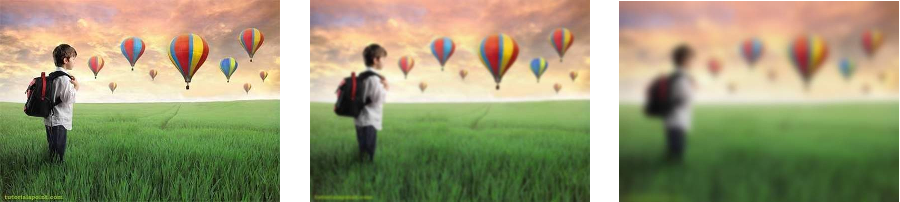
is called a smoothing operator. $S$ replaces each function value $f(\mathbf{x})$ by an average of the values of $f$ at the neighbors of $\mathbf{x}$, with weights given by the distribution $p$. Applying $S$ to the RGB-components of an image results in a blurred version of the image.
In Houdini the nodes called “Volume Blur” and “Volume Convolve $3\times 3 \times 3$” can be used to implements such an operator $S$, though only on functions $f$ defined on a bounded rectangle in $\mathbb{Z}^2$ or $\mathbb{Z}^3$. Such functions $f$ are called volumes in Houdini.
We call a family $a\mapsto S_a$ of smoothing operators parametrized by $a> 0$ a smoothing family if for all $C^0(\mathbb{Z}^n)$ we have
$$\lim_{a\to 0} S_a(f)=f.$$
Or equivalently, if the corresponding densities $p_a$ converge to
\begin{align*}\delta: \mathbb{Z}^n &\to \mathbb{R}\\\\ \delta(\mathbf{n})&= \delta_{0,\mathbf{n}}.\end{align*}
Here is the smooth version of the above theory: Consider the space
$$C^\infty_b(\mathbb{R}^n)= \{f\in C^\infty(\mathbb{R}^n) \,\,|\,\, f\text{ and all its partial derivatives are bounded} \}.$$
Suppose we have a probability density $p\in L^1(\mathbb{Z}^n)$ with mean zero. Then the linear map
\begin{align*}S: C^\infty_b(\mathbb{R}^n) \to C^\infty_b(\mathbb{R}^n) \\\\ (Sf)(\mathbf{x}) = \int_{\mathbb{R}^n} p(\mathbf{x}-\mathbf{y})f(\mathbf{y}) d\mathbf{y}\end{align*}
is called a smoothing operator. It is not hard to see that indeed $S_af$ is defined for all $C^\infty_b(\mathbb{R}^n)$ and is itself an element of $C^\infty_b(\mathbb{R}^n)$. Moreover, $S_a$ commutes with all partial derivatives:
$$\frac{\partial}{\partial x_j}\left(S(f)\right)= S\left(\frac{\partial f}{\partial x_j}\right).$$
Again, we call a family $a\mapsto S_a$ of smoothing operators parametrized by $a>0$ a smoothing family if for all $C^\infty_b(\mathbb{R}^n)$ we have
$$\lim_{a\to 0} S_a(f)=f$$
Here the limit means uniform convergence on compact subsets of $\mathbb{R}^n$ of $f$ and all its partial derivatives. The main difference to the $\mathbb{Z}^n$ case is that for the densities $p_a$ this now means convergence to a delta function. There is no need here to discuss delta functions, for in all calculations we will postpone taking the limit $a\to 0$ until the very end.
My (as everybody else’s) favorite smoothing family comes from the Gaussian distributions
$$p_a(\mathbf{x})=\frac{1}{(4\pi a)^{n/2}}\,\exp\left(\frac{|\mathbf{x}|^2}{4a}\right).$$
This family has the notable property that (interpreting the parameter $a$ as time) it solves the heat equation
$$\frac{\partial p_a}{\partial a}=\Delta p_a.$$
This can also be expressed as
$$S_a=\exp(a\Delta),$$
which implies that for all $a,b>0$ we have
$$S_{a+b}=S_a \circ S_b.$$
Let us now switch focus to the case $n=3$. There my second favorite smoothing family is given by
$$p_a(\mathbf{x}))=\frac{3a^2}{4\pi\sqrt{a^2+|\mathbf{x}|^2}^{\,5}}.$$
The reason I like this particular smoothing family comes from its relation to the Green’s operator
\begin{align*}G: C^\infty_0(\mathbb{R}^n) \to C^\infty_b(\mathbb{R}^n) \\\\ (Gf)(\mathbf{x}) = -\frac{1}{4\pi}\int_{\mathbb{R}^n} \frac{f(\mathbf{y})}{|\mathbf{x}-\mathbf{y}|}\,d\mathbf{y}\end{align*}
Quite often $G$ is denoted by $\Delta^{-1}$ because it is well-known that $G$ is a right-inverse of the Laplace-operator $\Delta$:
$$\Delta \circ G = \mbox{id}_{C^\infty_0(\mathbb{R}^n)}$$
It will be useful to have an approximation of $G$ without the singularity in the integrand: For $a>0$ define
\begin{align*}G_a: C^\infty_0(\mathbb{R}^n) \to C^\infty_b(\mathbb{R}^n) \\\\ (G_af)(\mathbf{x}) = -\frac{1}{4\pi}\int_{\mathbb{R}^n} \frac{f(\mathbf{y})}{\sqrt{a^2+|\mathbf{x}-\mathbf{y}|^2}}\,d\mathbf{y}\end{align*}
Theorem: With $S_a$ as defined earlier, we have
$$G_a = G\circ S_a= S_a\circ G.$$
Proof: The right equality follows from the easy to prove fact that $G$ commutes with all smoothing operators. Let $f$ be a function in $C^\infty_0(\mathbb{R}^n)$. Then $G_a(f)$ as well as $G\circ S_a(f)$ tend to zero at infinity. Since there are no nontrivial harmonic functions with this property, it is enough to ckeck the equation obtained by applying $\Delta$ to both sides of the left equation:
\begin{align*}\Delta\left(\mathbf{x}\mapsto-\frac{1}{4\pi}\int_{\mathbb{R}^n} \frac{f(\mathbf{y})}{\sqrt{a^2+|\mathbf{x}-\mathbf{y}|^2}}\,d\mathbf{y}\right) &=\left(\mathbf{x}\mapsto-\frac{1}{4\pi}\int_{\mathbb{R}^n}\Delta\left(\mathbf{x}\mapsto\frac{f(\mathbf{y})}{\sqrt{a^2+|\mathbf{x}-\mathbf{y}|^2}}\right)\,d\mathbf{y}\right)\\\\&= S_a(f).\end{align*}
$\blacksquare$
The smoke ring flow we have discussed so far applies to the limit of a fluid where all vorticity is concentrated in infinitely sharp vortex filaments (which can be described as closed space curves $\gamma$). In order to model realistic fluid flow, we have to give each filament a finite thickness $a$. This will be achieved by smoothing the singular velocity field generated by the infinitely sharp filament. This will be done in the next post, based on the above theory of smoothing.