Tutorial 7 – Obstacles

The Biot-Savart formula provides for a given set of curves \(\gamma = (\gamma_1,\ldots,\gamma_m)\) a divergence-free velocity field whose vorticity is concentrated along these curves. This led to a simple algorithm to model fluids on entire \(\mathbb R^3\). Here we present a way to treat obstacles.

Let \(\sigma\) be the boundary surface of an obstacle \(M\). Since the fluid cannot penetrate \(M\) the velocity field is tangent to \(\Sigma\). So we are searching for a divergence-free vector field \(u\) that is tangent to \(\Sigma\) and still has the correct vorticity. This amounts to solving a boundary value problem.

The Biot-Savart field \(u_{\gamma}\colon \mathbb R^3 \to \mathbb R^3\) (always smoothed a bit) is not tangent but has already the correct vorticity. Now if \(u_{\sigma}\colon \mathbb R^3 \setminus M \to \mathbb R^3\) is a divergence-free curl-free field and has the same normal component as \(u_{\gamma}\), then \(u_{\gamma} – u_\Sigma\) is tangent to \(\Sigma\) and still has the correct vorticity, i.e.\[u=u_{\gamma}-u_\Sigma\]solves the boundary value problem.

Though we cannot solve exactly for \(u_\Sigma\), we can approximate it.

Let \(\Sigma\) be a polygonal surface and consider its cells as smoke rings, \(\eta = (\eta_1,\ldots,\eta_n)\). Then we can compute strengths \(\Gamma_1,\ldots,\Gamma_n\) such that the flux of the Biot-Savart field \(u_\eta\) of \(\eta\) through each facet of \(\Sigma\) equals the the flux of \(u_\gamma\). This can be done by solving the following quadratic linear system:\[\sum_{i=0}^n\mathrm{flux}_{\eta_i}(u_{\eta_j})\Gamma_j = \mathrm{flux}_{\eta_i}(u_\gamma),\quad i,j\in \{1,\ldots,n\}.\]Since \(\eta_i\) are polygons the values \(\mathrm{flux}_{\eta_i}(u_{\eta_j})\) can be computed directly as a sum of ‘edge fluxes’,\[\mathrm{flux}_{\eta_i}(u_{\eta_j}) = \sum_{e\in \eta_i} \sum_{\tilde e\in\eta_j} \mathrm{edgeflux}(e,\tilde e),\]and there is an explicit formula to compute \(\mathrm{edgeflux}(e,\tilde e)\), which is implemented as method edge_flux in the following .h-file. Details can be found e.g. in the Steffen Weissmann’s thesis. How to include .h-files is explained here.

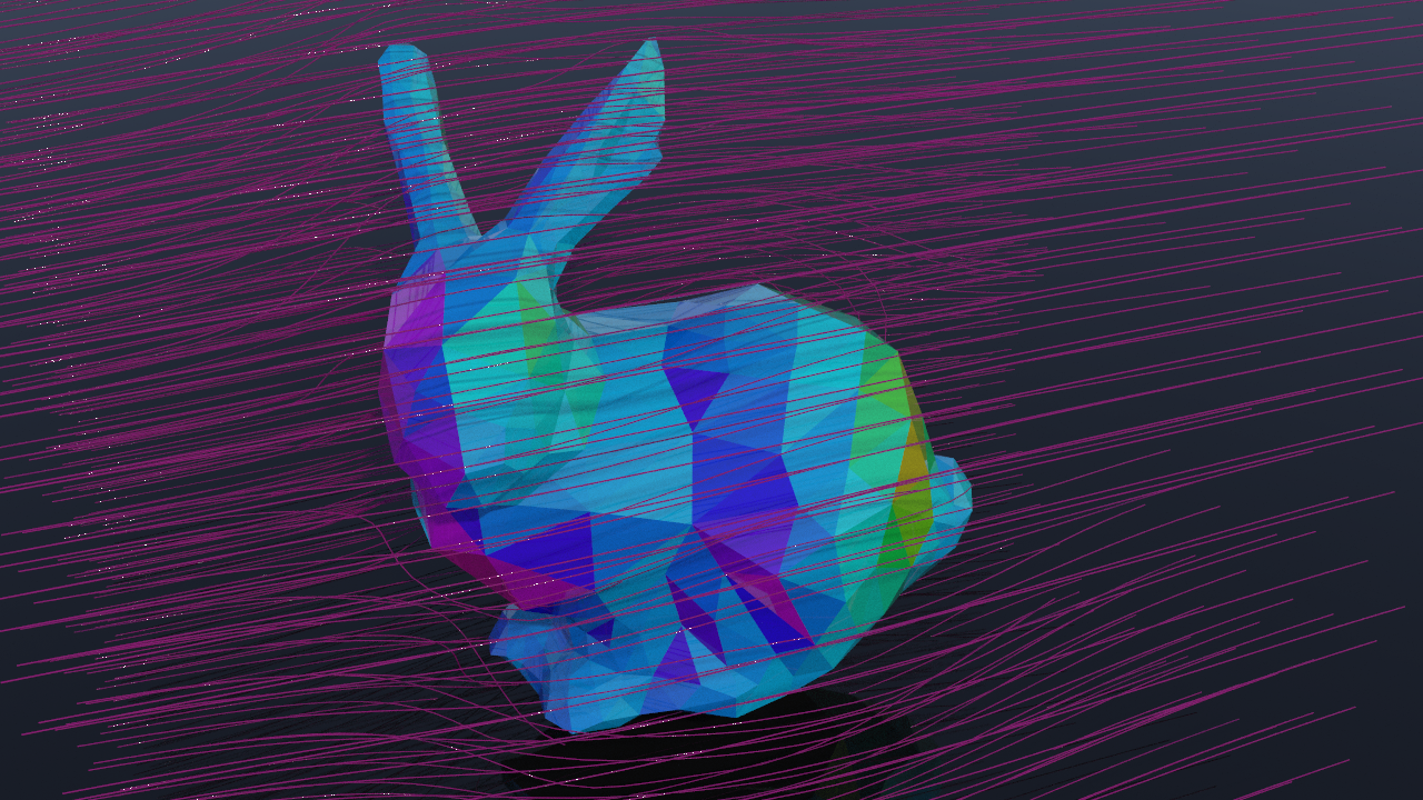
In this exercise we will use this technique to change a static constant field \(u_c = X \in \mathbb R^3\) to a field \(u\) that flows around \(\Sigma\).

The flux though a facet \(\varphi_i\) of \(\Sigma\) is then equal to the product of the area vector \(A\) and the vector \(X\): If \(\eta_i = \partial \varphi_i= (p_1,\ldots,p_k)\),\[\mathrm{flux}_{\eta_i}(u_c) = \langle A_i,X\rangle, \quad A_i = \tfrac{1}{2}\sum_{j=0}^k p_j\times p_{j+1}.\]Thus we have \(u = u_c – \sum_{i}\Gamma_i u_{\eta_i}\), where \(u_{\eta_i}\) denotes the smoothed Biot-Savart field and the coefficients \(\Gamma_i\) solve the following linear system\[\sum_{i=0}^n\mathrm{flux}_{\eta_i}(u_{\eta_j})\Gamma_j = \langle A_i,X\rangle.\]

All the fluxes can be computed in VEX. To solve the linear system we finally need Python. Therefore we can use a Python node with the following code

Here fluxmatrix is a global float[] attribute that contains the fluxes \(\mathrm{flux}_{\eta_i}(u_{\eta_j})\), i.e.\[\mathtt{fluxmatrix[i*n + j]} =\mathrm{flux}_{\eta_i}(u_{\eta_j})\]and A_X is a global float[] attribute containing the fluxes of \(u_c\), i.e.\[\mathtt{A\_ X[i]} =\langle A_i,X\rangle.\]

Homework (due 17 July). Write a network that, for a given vector \(X\in\mathbb R^3\) and a given surface \(\Sigma\) computes the corresponding velocity field \(u\). Visualize the integral curves of \(u\).