The velocity field of a fluid in \(\mathbb R^3\) (at rest at infinity) can be reconstructed from the vorticity by the Biot-Savart formula. Let us assume a fluid with vorticity concentrated along a filaments: Given a curve \(\gamma\colon \mathbb S^1 \to \mathbb R^3\) and \(a>0\), then the corresponding (smoothed) Biot-Savart field \(u_a\colon \mathbb R^3\to \mathbb R^3\) of \(\gamma\) (with smoothing parameter \(a\)) is given by \[u_a(p) = \frac{1}{4\pi}\int_{\mathbb S^1} \frac{(\gamma-p)\times d\gamma}{\sqrt{a^2+ |\gamma-p|^2}^3}.\]The field \(u_a\) is divergence-free with vorticity \(w_a=\mathrm{curl}\, u_a\) concentrated in a tube of radius \(a\) along \(\gamma\). \(w_a\) is obtained from \(\gamma\) by convolution with a certain smoothing kernel.
For \(a\to 0_+\) the vorticity \(w_a\) tends to the current given by integration over \(\gamma\): For \(v\colon \mathbb R^3 \to \mathbb R^3\) smooth with compact support, \[\lim_{a\to 0_+} \int_{\mathbb R^3} \langle v,w_a\rangle = \int_{\mathbb S^1} \langle v\circ\gamma,d\gamma\rangle.\]In the following we will suppress the dependency on the smoothing parameter \(a\).
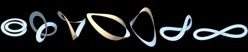
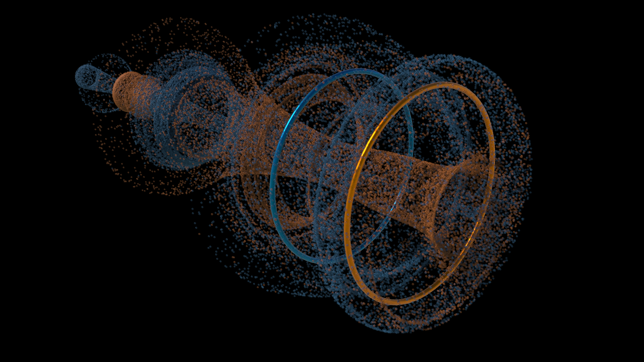
The vorticity is frozen in the fluid, i.e. \(\dot w + [u,w] = 0\). By the Biot-Savart formula we can reconstruct the velocity of the fluid only from its vorticity, this offers the possibility to approximate the whole fluid by advection of its vortex filaments, i.e. we just have to solve\[\dot\gamma = u\circ\gamma.\]This simple algorithm already enables us to reproduce certain phenomena – like e.g. leapfrogging smoke rings as shown in the picture above. All we need to know is the Biot-Savart field of a closed polygon.
Fortunately the Biot-Savart formula be explicitly integrated along straight edges: Given an (oriented) edge \(e\) parametrized by \(\eta\colon [0,1]\to \mathbb R^3\) with \(\eta(t) = q_1 + t(q_2-q_1)\), then \[u_e(p) =\frac{1}{4\pi}\int_0^1 \frac{(\eta-p)\times d\eta}{\sqrt{a^2+ |\eta-p|^2}^3}.\]Note that \(\eta^\prime = q_2-q_1\) and thus \((\eta-p)\times \eta^\prime = (q_1-p)\times (q_2-q_1)\) are constant. We have\[\frac{(\eta-p)\times \eta^\prime}{\sqrt{a^2+ |\eta-p|^2}^3} =\Bigl(\frac{\langle \eta – p, \eta^\prime\rangle \, (\eta – p)\times \eta^\prime}{\bigl(|\eta^\prime|^2 a^2 + |(\eta – p)\times\eta^\prime|^2\bigr)\sqrt{a^2 + |\eta – p|^2}}\Bigr)^\prime,\]where \((.)^\prime\) denotes the derivative with respect to the parameter \(t\). Thus we obtain an explicit formula for \(u_e\) in terms of the start and end point \(q_1\) and \(q_2\) of \(e\).
So, given a polygon \(\gamma\) we obtain the corresponding Biot-Savart field \(u\) by summing over the oriented edges of \(\gamma\). The picture bleow shows the integral curves of the Biot-Savart field of a discrete \(\gamma\) together with level sets of the solid angle function of \(\gamma\).
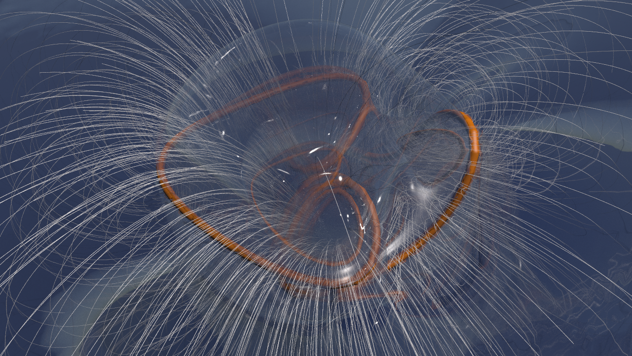
As expected the integral curves intersect the level sets orthogonally.
In general, given a set of discrete curves \(\gamma^1, \ldots, \gamma^m\), then we have \[u(p) = \sum_{\textit{edge e}} u_e(p),\]where \(u_e\) denotes the Biot-Savart field of the edge \(e\) and the sum runs over all (positively oriented) edges \(e\) in \(\gamma^1,\ldots,\gamma^m\).
Homework (due 3 July). Write a network that, for a given set of polygons, advects the vertices of the polygons by their own Biot-Savart field. Use a Runge-Kutta scheme and make it possible to move particles with the fluid.