![]()
Let \(M\subset \mathbb C\) be an open set and \(V\) a complex vector space with a non-degenerated complex-valued symmetric complex-bilinear form \(\langle.,.\rangle\). A null-curve is a map \(\gamma \colon M \to V\) such that\[\gamma^\ast\langle.,.\rangle = \langle d\gamma,d\gamma\rangle = 0\,.\]Unless explicitly stated differently \(\mathbb C^n\) is always equipped with its standard bilinear form\[\langle \psi,\psi\rangle = \sum_{i=1}^n \psi_i^2\,,\]which restricts to the standard inner product on \(\mathbb R^n\subset \mathbb C^n\).
Theorem. If \(\gamma\colon M \to \mathbb C^n\) is a holomorphic null-curve, then—away from the singular points of \(\gamma\)—the map \(f = \mathrm{Re}\,\gamma\) is a conformally immersed minimal surface.
Proof. Since \(\gamma\) is holomorphic, we have \(\gamma_y = i\gamma_x\). Thus we get \(\gamma_x = f_x -if_y\). The null-curve condition then yields\[0 = \langle \gamma_x,\gamma_x\rangle = |f_x|^2 – |f_y|^2 – 2i\langle f_x,f_y\rangle\]and thus \(|f_x|^2 = |f_y|^2\) and \(\langle f_x,f_y\rangle = 0\)—meaning that \(f\) is conformal. Moreover, as the real part of a holomorphic map, \(f\) is harmonic, which means that it is minimal. \(\square\)
Conversely, it is not hard to show that that—at least on a simply-connected domain \(M\)—each conformally immersed minimal surface comes from such a holomorphic null-curve. Moreover, the notion of a holomorphic null-curve extends in the obvious way to maps from a Riemann surface into a complex manifold with complex-bilinear fiber product.
Now let us equip \(\mathbb C^5\) with another bilinear form: For \(\psi=(\psi_1,\ldots,\psi_5) \in \mathbb C^5\), we set\[\langle\psi,\psi\rangle = \psi_1^2 +\psi_2^2 +\psi_3^2 -\psi_4\psi_5\,.\]This bilinear form restricts to an inner product of signature \((++++-)\) on \(\mathbb R^n\) and \(\mathcal L = \{\psi \in \mathbb C^5\setminus \{0\} \mid |\psi|^2 = 0\}\) is its complexified light-cone. Let furthermore \(\mathcal L_\ast\) denote the set of vectors in \(\mathcal L\) with non-vanishing last component,\[\mathcal L_\ast = \{\psi\in \mathcal L \mid \psi_5 \neq 0\} = \mathcal L \setminus (\mathbb C^4\times \{0\})\,.\]We define two maps:\[\sigma \colon \mathcal L_\ast \to\mathbb C^3,\quad \psi\mapsto \tfrac{1}{\psi_5}(\psi_1,\psi_2,\psi_3)\]and\[\tau \colon \mathbb C^3 \to \mathcal L_\ast,\quad x\mapsto (x,|x|^2,1)\,.\]One easily checks the following identities: Let \(\beta \colon \mathbb C^5 \to \mathbb C\) denote the projection to the 5th component, \(\beta(\psi) = \psi_5\), then \[\sigma\circ\tau = \mathrm{id}_{\mathbb C^3},\quad \tau\circ \sigma = \tfrac{1}{\beta}\mathrm{id}_{\mathcal L_\ast}\,.\]
Obviously the maps \(\sigma\) and \(\tau\) both preserve holomorphicity: If \(\varphi\colon M\to \mathcal L\) is holomorphic, then \(\gamma = \sigma\circ \varphi\) is meromorphic (holomorphic up to isolated points—the points for which \(\varphi\) hits \(\mathbb C^4\times\{0\}\)—where \(\gamma\) has poles). Conversely, any meromorphic \(\gamma\) appears from such a holomorphic \(\varphi\).
Lemma. \(\sigma^\ast \langle.,.\rangle = \beta^{-2}\langle.,.\rangle\) and \(\tau^\ast\langle.,.\rangle = \langle.,.\rangle\).
Proof. If \(\dot x \in T_x \mathbb C^3\), we have \(d\tau(\dot x) = (\dot x, 2\langle \dot x,x\rangle, 0)\). Thus \(|d\tau(\dot x)|^2 = |\dot x|^2\) and hence \(\tau^\ast\langle.,.\rangle\). Thus we get \[\sigma^\ast\langle.,.\rangle =\sigma^\ast\tau^\ast\langle.,.\rangle = (\tau\circ\sigma)^\ast\langle.,.\rangle\,.\]Now, if \(\dot\psi \in T_\psi \mathcal L_\ast\), we have \(d(\tau\circ \sigma)(\dot \psi) = d(\tfrac{1}{\beta})(\dot\psi) \psi +\tfrac{1}{\beta}\dot \psi\). From \(|\psi|^2=0\), we also get \(\langle\psi,\dot\psi\rangle = 0\) and thus\[|d\sigma(\dot \psi)|^2=|d(\tau\circ \sigma)(\dot \psi)|^2 = \langle d(\tfrac{1}{\beta})(\dot\psi) \psi+\tfrac{1}{\beta}\dot \psi,d(\tfrac{1}{\beta})(\dot\psi)\psi+\tfrac{1}{\beta}\dot \psi\rangle = \tfrac{1}{\beta^2}\langle \dot\psi,\dot\psi\rangle\,.\]Hence \(\sigma^\ast\langle.,.\rangle = \beta^{-2}\langle.,.\rangle\). \(\square\)
Corollary. \(\sigma\) and \(\tau\) both preserve null-curves.
So we have seen that conformally immersed minimal surfaces in \(\mathbb R^3\) can be identified with null-curves in \(\mathbb C^3\) or \(\mathcal L\). Thus, if we find families of null-curves, we find families of minimal surfaces. An obvious such family is obtained by the action of \(\mathbb S^1\) on the complex vector space—this yields the so called associated family.
Lemma. If \(\varphi\colon M \to V\) is a holomorphic null-curve and \(c\in \mathbb S^1\subset\mathbb C\), then \(\varphi_c = c\varphi\) is a also a holomorphic null-curve.
Proof. We have \(d\varphi_c = c\, d\varphi\). Thus \(|\varphi_c|^2 = c^2|\varphi|^2=0\), i.e. \(\varphi_c\) is a null-curve. Since scalar multiplication by a constant is complex linear, holomorphicity is preserved as well. \(\square\)
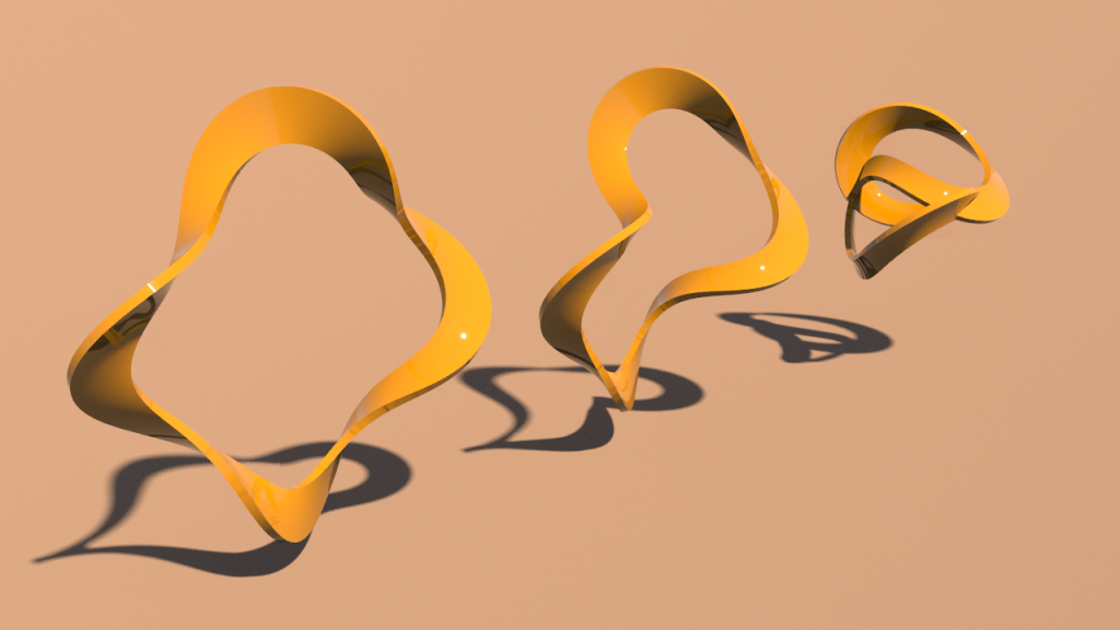
The Kusner surfaces are obtained as the real part of the \(\mathbb C^3\)-valued meromorphic curve\[\gamma = \frac{i}{z^{2p}-1+rz^p}\Bigl(z^{2p-1} – z, -i(z^{2p-1} + z), \tfrac{p-1}{p}(z^{2p} +1)\Bigr)\,.\]where \(p\in \mathbb N\), \(r = 2\sqrt{2p-1}/(p-1)\) and \(z \colon \mathbb S^2 \to \mathbb C\) denotes the stereographic projection. One checks that \(\gamma\) is a null-curve. By the lemma above we can easily visualize its associated family by a slight modification of the last exercise.
Another source of families is the group of complex linear transformations that preserve the bilinear form: For \(V\) complex vector space with non-degenerate bilinear form \(\langle.,.\rangle\), then\[O(V) = \{A\in\mathrm{GL}(V)\mid \langle A\psi,A\tilde\psi\rangle = \langle\psi,\tilde\psi\rangle\quad \forall \psi,\tilde\psi\in V\}\,.\]The proof of the next lemma is almost identical to the last one. We omit it.
Lemma. Let \(\varphi\colon M \to V\) be a holomorphic null-curve, \(A\in O(V)\), then \(\tilde\varphi :=A\varphi\) is also a holomorphic null-curve.
We want to apply this to the Kusner surfaces. Therefore we first construct a lift \(\varphi\colon M \to \mathcal L\) of the Kusner null-curve \(\gamma\colon M \to \mathbb C^3\) above and then apply a linear transformation in \(\mathbb C^5\) preserving \(\mathcal L\). We make the following ansatz: For \(\rho\in \mathbb C\),\[\varphi =\Bigl(i(z^{2p-1} – z), (z^{2p-1} + z), i\tfrac{p-1}{p}(z^{2p} +1),\alpha(z),\rho(z^{2p}-1+rz^p)\Bigr)\,,\]where \(\alpha\) is a polynomial in \(z\) such that \begin{align*}\alpha(z) \rho(z^{2p}-1+rz^p) & = -(z^{2p-1} – z)^2 + (z^{2p-1} + z)^2 – (\tfrac{p-1}{p})^2(z^{2p} +1)^2\\ & =4z^{2p} – (\tfrac{p-1}{p})^2(z^{4p} +2z^{2p} +1)\\ & = – (\tfrac{p-1}{p})^2(z^{4p} +2(1-2\tfrac{p^2}{(p-1)^2})z^{2p} +1) \\& = – (\tfrac{p-1}{p})^2(z^{4p} +2\tfrac{1-2p-p^2}{(p-1)^2}z^{2p} +1)\,.\end{align*}On the other hand, we have\begin{align*}(z^{2p}-1 + rz^p)(z^{2p}-1 – rz^p) & = (z^{2p}-1)^2 – r^2z^{2p} \\ & = z^{4p} – (2+r^2)z^{2p} + 1 \\ & =z^{4p} – 2(1+2\tfrac{2p-1}{(p-1)^2})z^{2p} + 1\\ & = z^{4p} + 2\tfrac{1 – 2p – p^2}{(p-1)^2} z^{2p} + 1\end{align*}Thus we can set \(\rho = \tfrac{p-1}{p}\) and \(\alpha(z)=-\tfrac{p-1}{p}(z^{2p}-1 – rz^p)\) and obtain the following formula for the holomorphic null-curve:\[\varphi = \Bigl(i(z^{2p-1} – z), (z^{2p-1} + z), i\tfrac{p-1}{p}(z^{2p} +1),\tfrac{p-1}{p}(rz^p + (z^{2p}-1)),\tfrac{p-1}{p}(rz^p – (z^{2p}-1))\Bigr)\,.\]If we now apply a coordinate change \[e_1 \to e_1,\quad e_2\to e_2, \quad e_3\to e_3, \quad e_4 \to e_5 – e_4, \quad e_5 \to e_5 + e_4\,,\] then the bilinear form \(\langle.,.\rangle\) takes the form \[\langle \psi,\psi\rangle = \psi_1^2 + \psi_2^2 + \psi_3^2 + \psi_4^2 – \psi_5^2\] and is preserved by real rotation matrices mixing the first 4 components, as e.g. \[\begin{pmatrix}1 & 0 & 0 & 0 & 0 \\ 0 & \cos t & 0 & -\sin t & 0 \\0 & 0 & 1 & 0 & 0 \\ 0 & \sin t & 0 & \cos t & 0 \\ 0 & 0 & 0 & 0 & 1 \\\end{pmatrix},\quad t\in \mathbb R\,.\]If we apply it to the holomorphic null-curve which, after the coordinate change, looks as follows\[\tilde \varphi =\Bigl(i(z^{2p-1} – z), (z^{2p-1} + z), i\tfrac{p-1}{p}(z^{2p} +1),\tfrac{p-1}{p}(z^{2p}-1),\tfrac{p-1}{p}rz^p\Bigr)\]we obtain new a family of minimal surfaces. The \(\mathbb C^3\)-valued null-curve takes the form\[\gamma = \tfrac{1}{\tilde\varphi_5 – \tilde\varphi_4}(\tilde\varphi_1,\tilde\varphi_2,\tilde\varphi_3)\,.\]Here a sequence of members in the corresponding family:
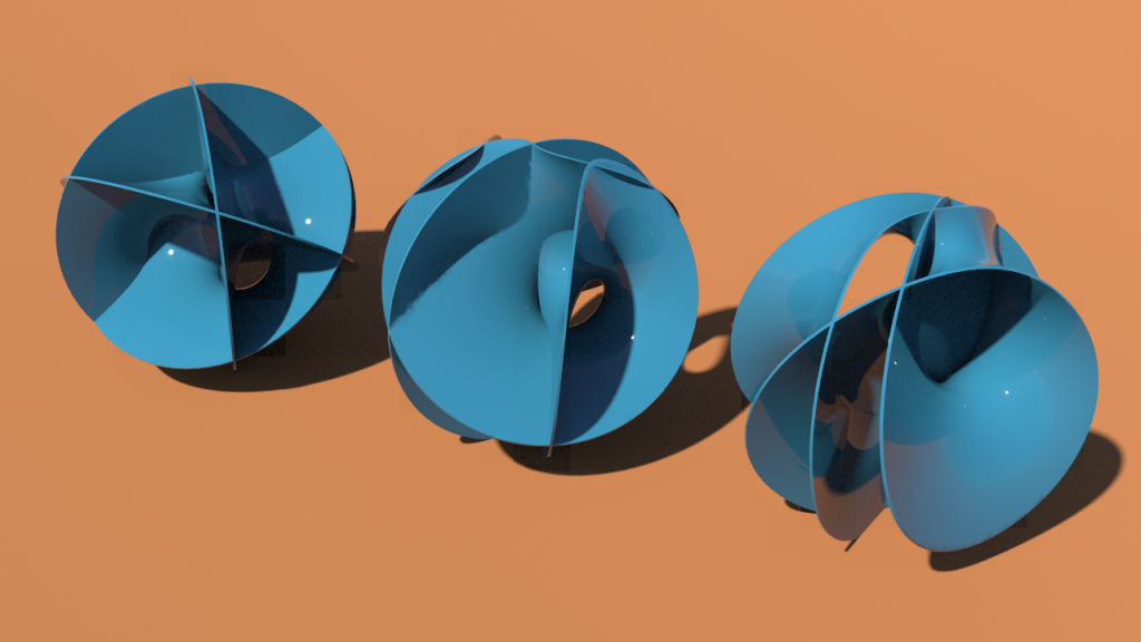
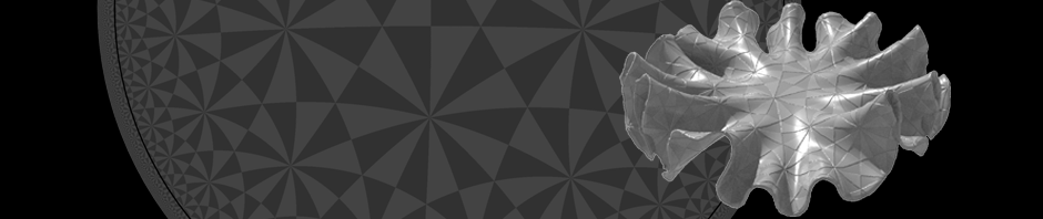
The minimal surfaces have planar ends at the singularities. The pictures above show the part of the surface contained in a sphere of fixed radius. To achieve this, one can use the boolean sop node which allows to intersect a surface with the interior of a sphere. Make sure here that input A is treated as surface and input B is treated as volume.
Unfortunately, the node will produce artefacts unless we cut away vertices which are mapped to points whose magnitude is too large. Fortunately, there is a node to fix this. It is called Polycut and allows us to delete vertices on which a specified attribute exceeds a certain value (parameters should be set to Type: Points, Strategy:Remove, DetectEdgeChanges:Cut At Attribute Change). So we can just store the magnitude as an attribute on points (by a point wrangle node) and then use Polycut to remove all points which lie too far outside the ball we want to intersect the surface with.
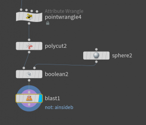
Then intersect by a boolean node. There we select to generate a primitive group A Inside B so that we can delete everything else which which is not in this group using a blast node.
Homework (due 21 May): Wire up a network that visualizes (by two interactive parameters) the associated and an additional family of Kusner’s minimal surfaces.