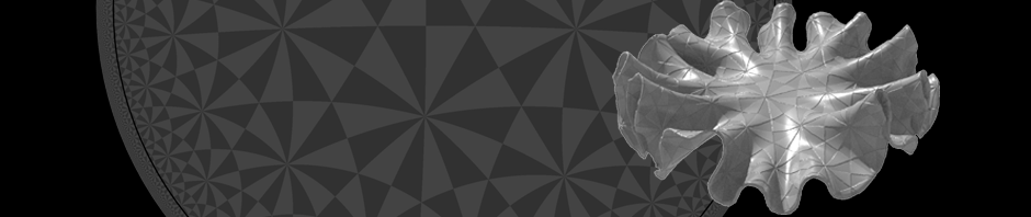
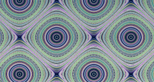
 The above picture shows examples of K-surfaces, i.e. surfaces with constant Gaussian curvature $K=-1$. The picture was made by Nicholas Schmitt and is part of the GeometrieWerkstatt Gallery. Instead of writing at length about the theory of K-surfaces and their relation to hyperbolic Geometry and the discrete Pendulum equation (as discussed in the class) , I will refer here to lecture notes of a course I gave at Beiing University in 2009.
Discrete K-surfaces
Posted in Uncategorized
Leave a comment
Tutorial 12: The Pendulum
A pendulum is a body suspended from a fixed support so that it swings freely back and forth under the influence of gravity. A simple pendulum is an idealization of a real pendulum—a point of mass \(m\) moving on circle of radius \(\ell\) under the influence of a uniform uniform gravity field of strength \(g\) pointing down.
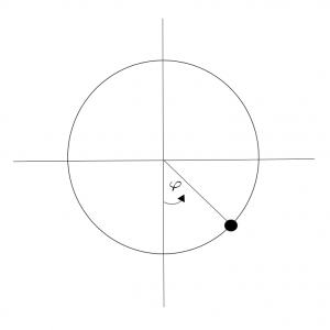
Its position is described by an angular coordinate \(\varphi\) and its energy is the sum of kinetic energy \(\tfrac{m}{2}\ell^2 \dot\varphi^2\) and gravitational potential energy \(-m\ell g\cos \varphi\):\[E(\varphi,\dot\varphi) = \tfrac{m}{2}\ell^2\dot\varphi^2 – m\ell g\cos\varphi\,.\]Its motion is then described by the following differential equation: \[\ddot\varphi = -\tfrac{g}{\ell}\sin \varphi\,.\]One easily checks that energy is a constant of motion,\[\dot E = m \ell^2\dot \varphi \ddot\varphi + m\ell g \dot\varphi\sin\varphi =-m \ell\dot \varphi g\sin\varphi + m\ell g \dot\varphi\sin\varphi = 0\,.\] Here a picture of the corresponding energy levels in phase space.
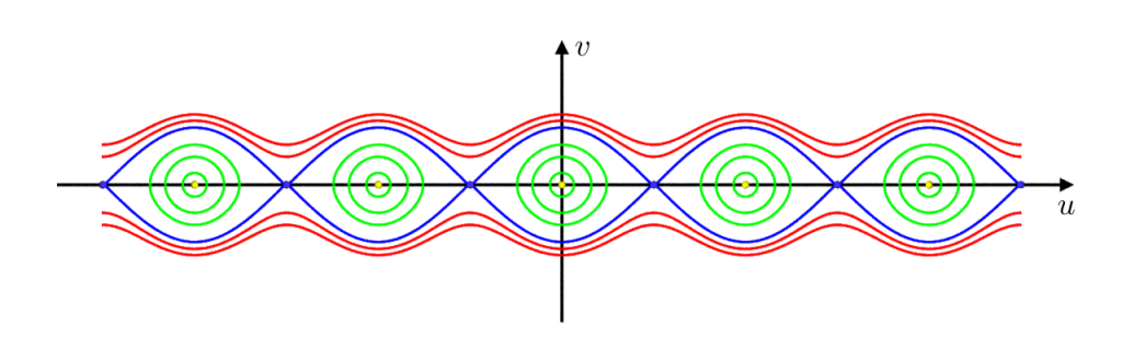
In the following we will set \(m=g=\ell=1\).
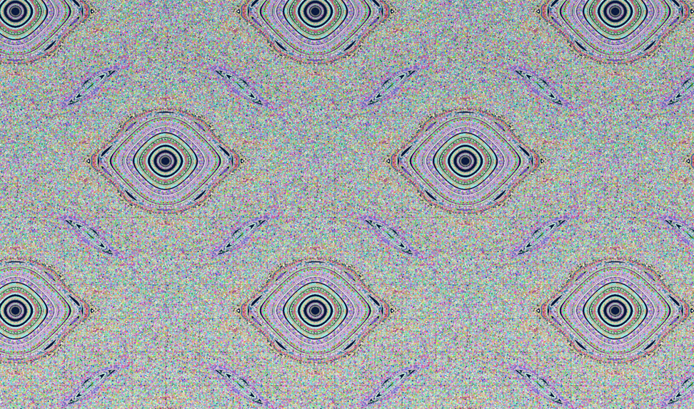
The simple pendulum is what is called an integrable Hamiltonian system. Now, if we discretize \(\ddot \varphi\) with timestep \(\varepsilon>0\) according to the Verlét we obtain the following recursion:\[\begin{pmatrix}\varphi_{n+1}\\ \varphi_n\end{pmatrix} = \sigma\begin{pmatrix} \varphi_n\\ \varphi_{n-1}\end{pmatrix} \mod 2\pi \mathbb Z^2\,,\]where \(\sigma\colon \mathbb R^2 \to \mathbb R^2\) is given by\[\sigma\begin{pmatrix} \varphi_n\\ \varphi_{n-1}\end{pmatrix} :=\begin{pmatrix} 2\varphi_n – \varphi_{n-1} – K \sin(\varphi_n) \\\varphi_n\end{pmatrix},\quad K = \varepsilon^2\,.\]The map \(\sigma\) is the well-known Chirikov standard map—an area-preserving (i.e. symplectic) map, which shows chaotic behavior. As such it serves as an important model in chaos theory.
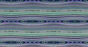
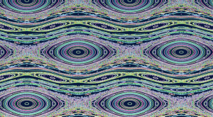
Here \(K=0.2,0.5,0.7,0.9\) from top to bottom.
The phase space is not ordered anymore by the constants of motion. Though order is not totally gone. The chaotic regions cannot diffuse over the whole phase space but are bounded by so-called KAM orbits. As guaranteed by Kolmogorov–Arnold–Moser (KAM) theory, a non-neglectable amount will survive for small perturbations.
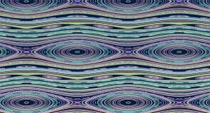
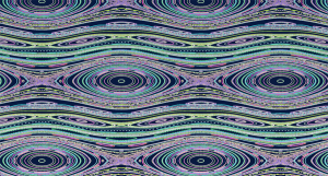
Remarkably, if we use \(4\arg(1+Ke^{-i\varphi})\) instead of \(\sin\varphi\) in the iteration we again obtain an integrable system. How to get to this discrete version of \(\sin\) in this article. It also provides a formula for the constant of motion.
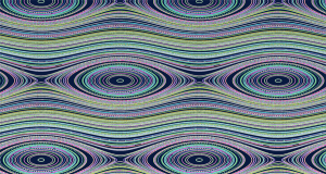
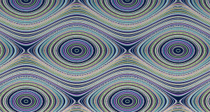
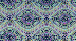
Here again \(K=0.2,0.5,0.7,0.9\) from top to bottom.
To produce these pictures in Houdini one can just randomly seed a bunch of particles on a the square \(M=[-\pi,\pi]^2\), color it randomly and iterate by a solver node. To visualize the whole sequence one can keep track of the history using a trail node. Though if we want to play around with parameters that is not an optimal setup. One better uses a loop with feedback—only one has to remember the point positions in each iteration.
Here is a way to do this: In the \((k+1)\)st iteration we extract the points of the \(k\)th iteration by a delete node. Then we apply the iteration formula and merge again with all previous points. Since the merge node just appends the points we can extract using a delete node. The network thus might look as follows.
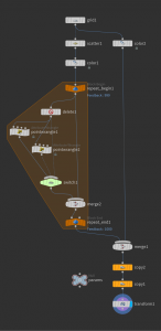
The copy and transform nodes at the end are used to copy the fundamental domain in \(x\)- and \(y\)-direction—just for visualization purposes.
Homework (due 9 July). Build a network that visualizes the orbits of the pendulum equation. It shall be possible to specify \(K\), the number of orbits and the total number of iterations (resolution of the obits). Use a checkbox parameter to choose between \(\sin\) and its discrete counterpart.
Posted in Tutorial
Leave a comment
Tutorial 11: CMC Snails, Tires and Soap Bubbles
In previous tutorials we compute immersed minimal surfaces. These immersions were the critical points of Dirichlet energy. You have seen in the lecture that, if we additionally include a volume constraint, then the critical points have no longer mean curvature \(H=0\) but it is constant—we obtain so called constant mean curvature (CMC) surfaces.
Let \(M\) be a surface. On the space of immersion \(f\colon M\to \mathbb R^3\) we consider for fixed \(p \in \mathbb R\) the energy\[\mathbf E_p(f) = E_D (f) + p V(f)\,,\]where\[E_D(f)= \tfrac{1}{2}\int_M |df|^2,\quad V(f) = \tfrac{1}{6}\int_M \langle f, df\times df\rangle\,,\]i.e. \(E_D(f)\) is the Dirichlet energy of \(f\) and \(V(f)\) the volume ‘enclosed’ by \(f\).
If we look at the critical points of \(\mathbf E_\lambda\) we find that these are CMC immersions: As seen in the lecture, we have\[ \dot{E}_D = \int_M \langle -\Delta^g f,\dot f\rangle,\quad \dot V = \int_M \langle N,\dot f\rangle\,.\]Moreover, \(\Delta^g f = -2HN\). Thus\[\mathrm{grad}_f\,\mathbf E_p = -\Delta^g f + p N = (2H +p) N\,.\]Thus a critical point \(f\) satisfies \(H = -p/2\).
So if we minimize for a given fixed \(p\) the energy \(\mathbf E_\lambda\) we obtain a CMC surface. One way to minimize is gradient descent. As explained in this fabulous article another and actually better method to minimize is the so-called momentum method—it guarantees faster convergence. So we are left to solves the following second order equation\[\ddot f + \rho\dot f = \Delta^g f + p N\,\]for some damping constant \(\rho>0\).
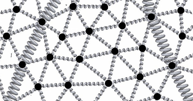
The equation above also has a nice Newtonian interpretation: By Newtons second law the above equation describes a surface on which act two forces—surface tension \(\Delta^g f\) and pressure \(pN\).
For the second derivative we use the same ansatz as last time and the first derivative is approximated by a difference quotient: For given stepsize \(\varepsilon >0\),\[\frac{f(t+\varepsilon) – 2f(t) +f(t-\varepsilon)}{\varepsilon^2} + \rho\frac{f(t) –f(t-\varepsilon)}{\varepsilon} = \Delta^{g(t)} f(t) + \lambda N(t)\,.\]Rearranging terms yields\[f(t+\varepsilon) =\varepsilon^2 \bigl(\Delta^{g(t)} f(t) +\lambda N(t)\bigr) +2f(t) – f(t-\varepsilon) – \rho\varepsilon (f(t)-f(t-\varepsilon))\,.\]Note that here—in contrast to last time—the Laplace operator depends on \(t\) as well.
One might be tempted to approximate the first derivative by a more symmetric expression like the average of difference quotients, but this is doomed. As Albert explained to me, that’s well known—e.g. if one discretizes the left hand side of the diffusion equation \(\dot u = \Delta u\) by the average of difference quotients the system becomes unconditionally unstable, i.e. no matter what \(\varepsilon\) one chooses the equation is unstable.
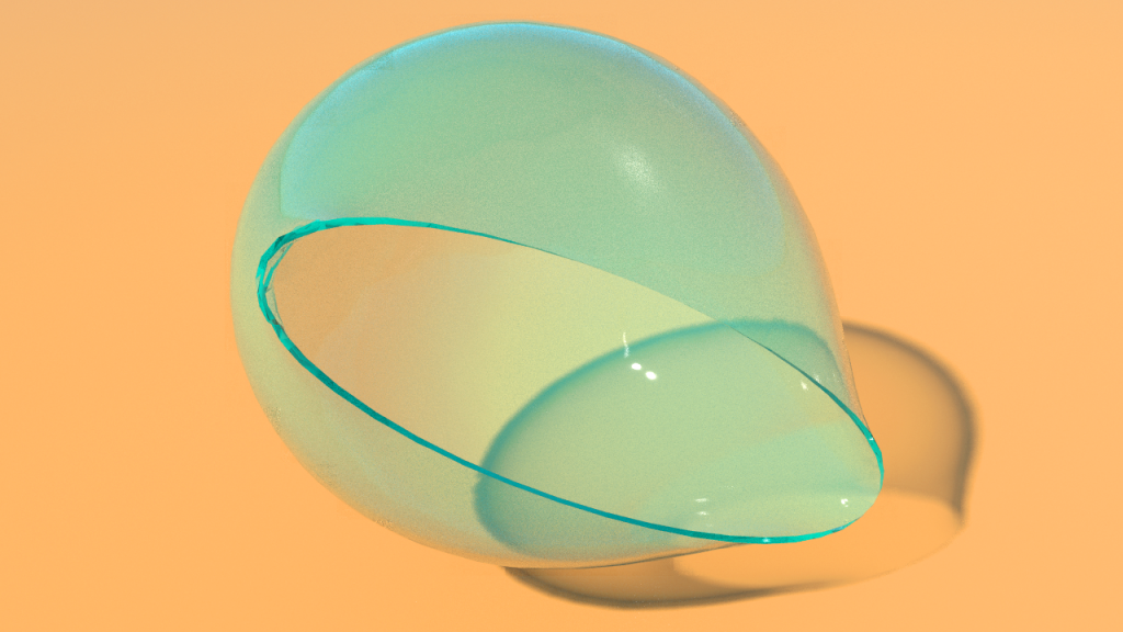
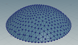
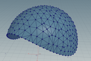
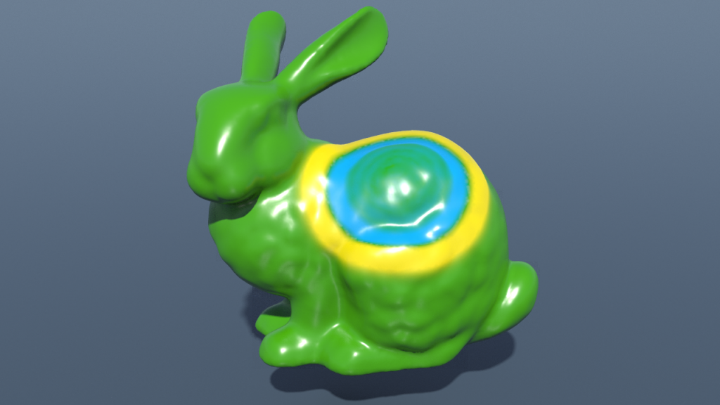
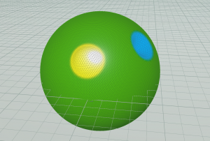
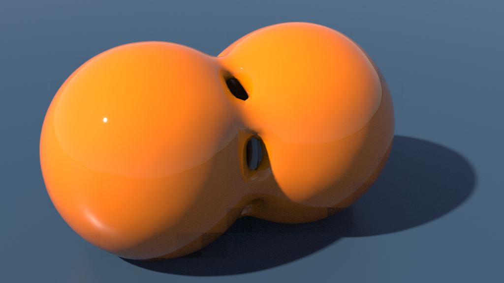
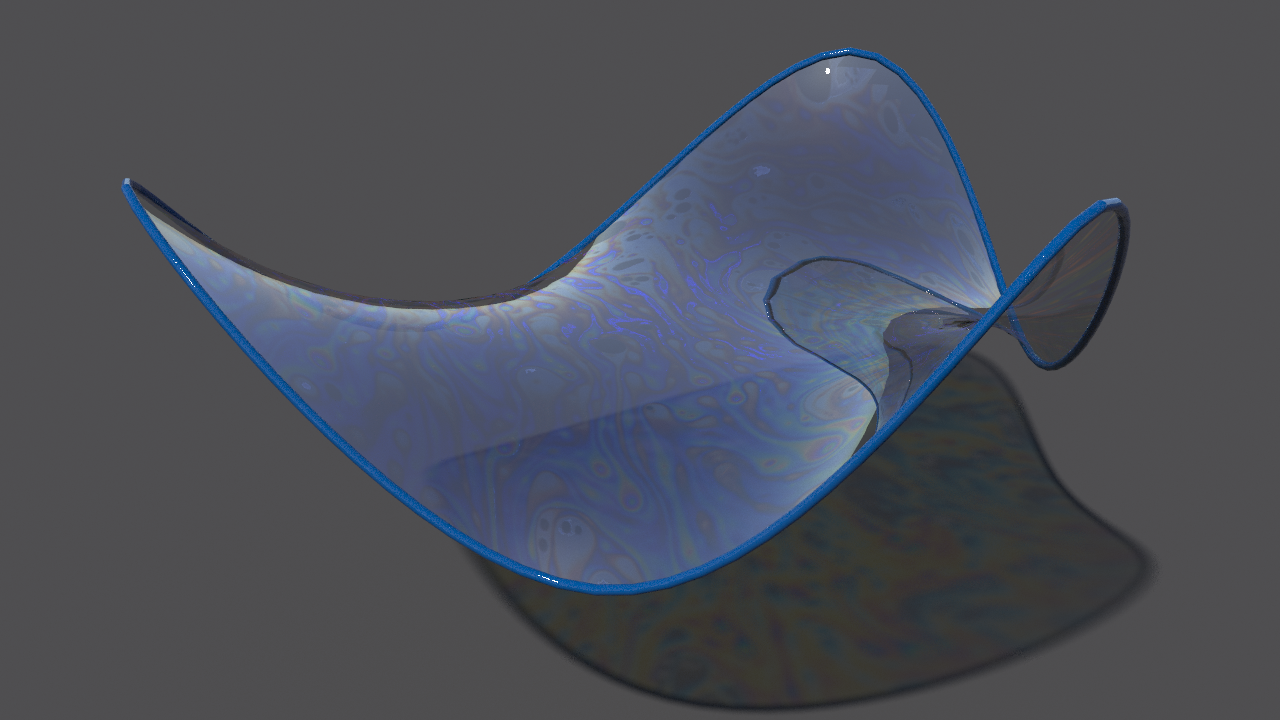
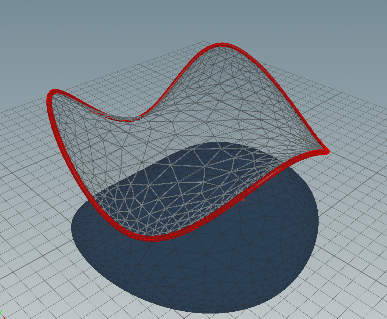
Let \(M\) be a surface with boundary. Minimization of \(E_p\) for a suitably chosen pressure \(p\) among all immersions which have the same boundary curve \(\gamma\) seems to work quite nicely. E.g. a flat disk is flowing to a spherical cap as show in the picture below.
As a short video shows, the method converges quickly.
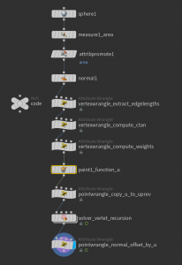
Here the corresponding network—it just prepares the initial conditions and implements the flow using a solver node.
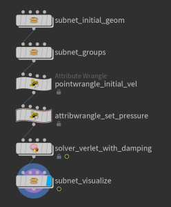
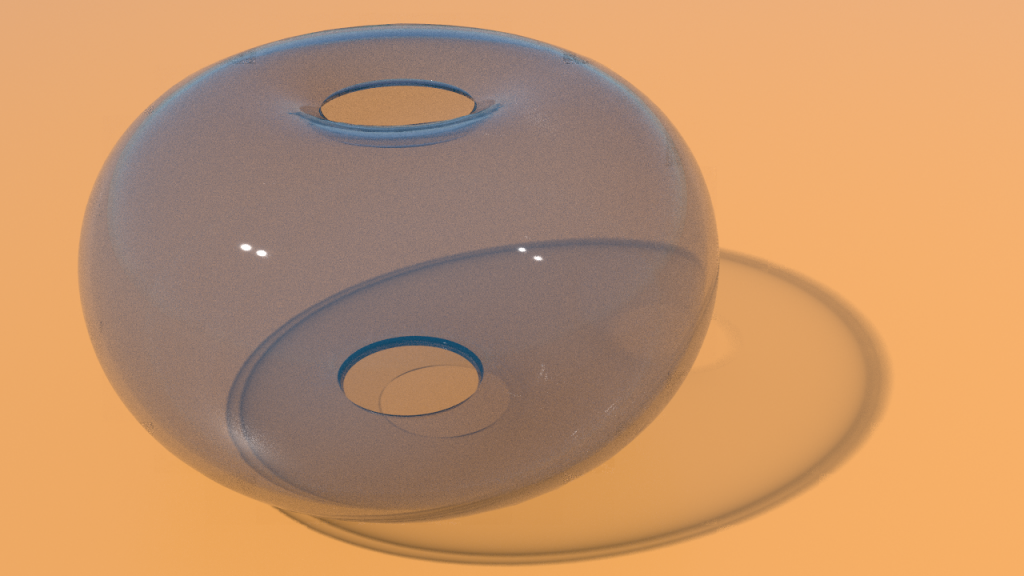
More interestingly, this also works for more generic boundary curves producing CMC surface which are no longer a part of a sphere.
In principle triangles can degenerate during the flow. To prevent them from becoming too bad we just used a polydoctor node (inside the solver) to repair the mesh if it becomes necessary. Not all situations can be fixed this way but it often help a lot.
For small pressure \(p\) the surface tension and pressure can balance and we end up with a CMC surface. For large \(p\) this is no longer true and the surface just blows up—we just pump more and more air ‘into’ the surface.
From physics we know that pressure is not constant—the ideal gas law says that, up to physical constants,\[pV = T,\]where \(T\) denotes temperature. It is worth to look at the dynamics one gets if we fix \(T\) and include the dependence of \(p\) on \(V\) in the force. Here a movie of an ellipsoid with some downward pointing impulse moving according to the equations of motion.
Let us come back to the problem of computing CMC surfaces. Therefore let us now impose a hard volume constraint, i.e. we minimize Dirichlet energy over all immersions which satisfy\[C(f) := V(f) – V_0 = 0\] for a given fixed \(V_0\in \mathbb R\). Such constraint optimization problems can be tackled by the so-called augmented Lagrangian method (ALM). Here \(\lambda\) is modified during the minimization: For a given initial \(\lambda\in \mathbb R\) iterate
- for fixed \(\lambda\), minimize the unconstraint problem\[\mathbf E_{aug}(f) = E_D(f) + \tfrac{1}{2}C(f)^2 +\lambda C(f)\,,\]
- use the minimizer \(f_0\) to update \(\lambda\) \[\lambda \gets \lambda + C(f_0)\,.\]
If we don’t minimize to the very end in the first step, but instead change it to a finite amount of gradient descent, and interpret the update of \(\lambda\) as a forward Euler step we obtain the continuous system:\begin{align*}\dot f & = \Delta^g f – (\lambda+C(f)) N\,,\\ \dot \lambda &=C(f)\,,\end{align*}where \(N\) denotes the Gauss map of \(f\)—which is the gradient of the volume functional \(V\).
Now let us look at a stationary point \(f\) of this continuous system: \(\dot \lambda = 0\) implies that \(V(f) = V_0\). From \(\dot f = 0\) then follows \(0 = \Delta^g f – \lambda N\). Thus we have\[2H\, N = -\Delta^g f = -\lambda N\,.\]So a stationary point \(f\) is just a CMC surface with mean curvature \(H=-\lambda/2\).
Let us again change the first line of the system above to second order with damping. The final system then becomes\begin{align*}\ddot f + \rho\dot f & = \Delta^g f – (\lambda + C(f)) N\,,\\ \dot \lambda &=C(f)\,,\end{align*}for some damping constant \(\rho>0\). Again the stationary points are CMC.
So, for a given stepsize \(\varepsilon >0\), we finally do the following updates: \[f(t+\varepsilon) = \varepsilon^2 \bigl(\Delta^{g(t)} f(t) – (\lambda(t)+C(f(t))) N(t)\bigr) +2f(t) – f(t-\varepsilon) – \rho\varepsilon(f(t)-f(t-\varepsilon))\,,\]followed by\[\lambda(t+\varepsilon) = \lambda(t) + \varepsilon C(f(t+\varepsilon))\,.\]
This all translates nicely to the discrete case–the Laplace operator is given by cotangent weights and the gradient the volume is the vertex normal field \(N\) which at a vertex \(i\) is given by the area vector of the boundary of the vertex star (the \(1\)-link), i.e. if \(j_1,\ldots,j_n=j_0\) denote the neighboring vertices of \(i\) ordered counter-clockwise, then\[N_i = A_i/|A_i|, \textit{ where } A_i = \tfrac{1}{2}\sum_{k=0}^{n-1} (f_{j_k}-f_i)\times (f_{j_{k+1}} – f_i)\,.\]
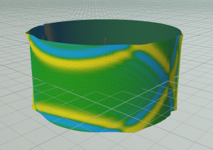
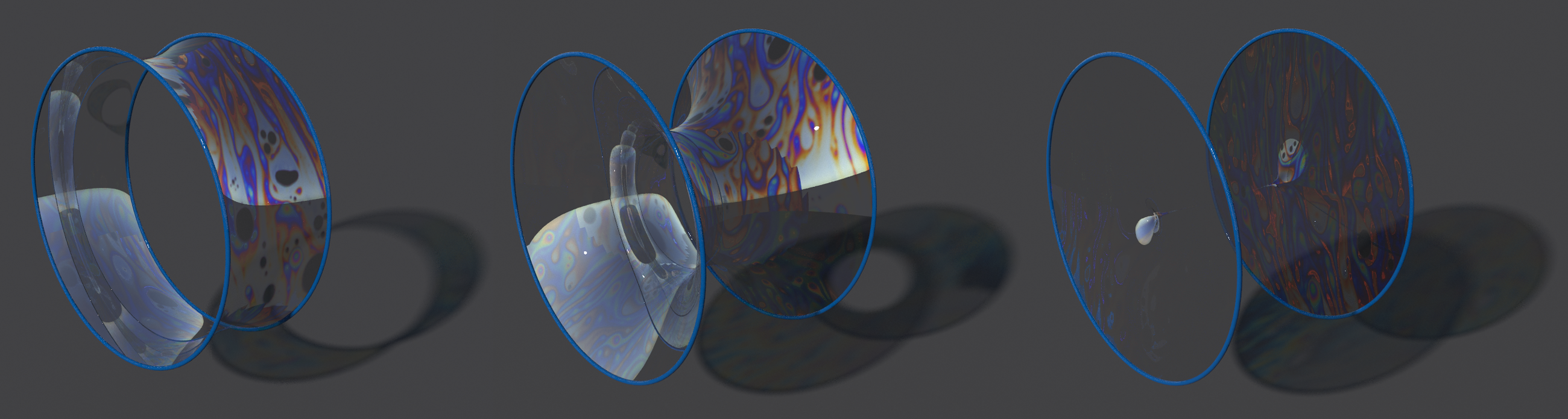
Here a movie of the dynamics of a flat ellipsoid blowing up to the CMC surface in the teaser image. The method is not restricted to disks. Below you find an image of a CMC cylinder.
Homework (due 2 July). Build a network which flows a given surface to a CMC surface of prescribed volume.
Posted in Tutorial
Leave a comment
Symplectic Maps and Flows
Consider a physical system consisting of $k$ massive particles at positions in $\mathbb{R}^3$ which we can assemble in a vector in $\mathbf{q}\in\mathbb{R}^m$ where $m=3k$. Likewise, the velocities of these particles at a given instant of time can be described by a vector $\mathbf{v}\in\mathbb{R}^m$. The corresponding linear momentum then is the vector
$$\mathbf{p}=M\mathbf{v}$$
where $M\in \mathbb{R}^{m\times m}$ is a diagonal matrix with entries (partitioned into triples of equal consecutive entries) that record the masses of the particles. At each instant of time the state of the system is then given by a vector
$$\left(\begin{array}{c}\mathbf{p}\\\mathbf{q}\end{array}\right)\in \mathbf{R}^{2m}.$$
The evolution of the system is described by a smooth map
$$\mathbf{q}:\mathbb{R}\to\mathbb{R}^m.$$
Suppose that the only forces acting on the particles come from a fixed potential energy function $U:\mathbb{R}^m\to \mathbb{R}$, so the potential energy of the system in position $\mathbf{q}$ is $U(\mathbf{q})$. Then Newton’s laws tell us that the position $\mathbf{q}(t), t\in [a,b]$ evolves according to the equation of motion
$$M\ddot{\mathbf{q}} = -\mbox{grad}_{\mathbf{q}}\,U$$
For the state vector $\left(\begin{array}{c}\mathbf{p}\\\mathbf{q}\end{array}\right)$ this amounts to the first order differential equation
$$\left(\begin{array}{c}\mathbf{p} \\ \mathbf{q}\end{array}\right)^{\!\small\bullet}=\left(\begin{array}{c}-\mbox{grad}_{\mathbf{q}}\,U \\ M^{-1}\,\mathbf{p}\end{array}\right).$$
We view the right-hand side as a vector field $V:\mathbb{R}^{2m}\to \mathbb{R}^{2m}$ with
$$V\left(\begin{array}{c}\mathbf{p} \\ \mathbf{q}\end{array}\right)=\left(\begin{array}{c}-\mbox{grad}_{\mathbf{q}}\,U \\ M^{-1}\,\mathbf{p}\end{array}\right).$$
This particular vector field has striking special properties, but before discussing these let us switch to a more general context: Suppose $n\in \mathbb{N}$ and let $V:\mathbb{R}^n\to\mathbb{R}^n$ be a smooth vector field. Suppose that for all $\mathbb{x}\in \mathbb{R}^n$ the initial value problem
\begin{align*}\gamma(0) &=x \\\\ \dot{\gamma}(t)&=V_{\gamma(t)}\end{align*}
has a solution $\gamma:\mathbb{R}\to\mathbb{R}^n$. Then for all $t\in \mathbb{R}$ we can define the flow maps
$$g_t:\mathbb{R}^n\to \mathbb{R}^n$$
by the property that
$$g_0 =\textrm{id}_{\mathbb{R}^n}$$
and for all $x\in \mathbb{R}^n$ and $t\in \mathbb{R}$ we have
$$\frac{d}{d\tau}{\large|_{\tau=t}}\,\,g_\tau(x)=V_{g_t(x)}.$$
Now we are ready to give the definitions needed for understanding what is special about the vector field $V$ that we started with. We begin with some Linear Algebra:
Let $J$ denote the following $2m\times 2m$ matrix:
$$J=\left(\begin{array}{c} 0 & -I \\ I & 0\end{array}\right).$$
Definition 1: The skew-symmetric bilinear form
\begin{align*}\sigma:\mathbb{R}^{2m} \times \mathbb{R}^{2m}\to \mathbb{R} \\\\ \sigma(\mathbf{u},\mathbf{v})=\langle J\mathbf{u},\mathbf{v}\rangle = -\mathbf{u}^t J \mathbf{v}\end{align*}
is called the standard symplectic form on $\mathbb{R}^{2m}$.
Definition 2: A matrix $A\in \mathbb{R}^{2m\times 2m}$ is called symplectic if for all $\mathbf{u},\mathbf{v}\in\mathbb{R}^{2m}$ we have
$$\sigma(A\mathbf{u},A\mathbf{v})=\sigma(\mathbf{u},\mathbf{v})$$
or equivalently, if
$$A^t JA=J.$$
Definition 3: A matrix $Y\in \mathbb{R}^{2m\times 2m}$ is called infinitesimally symplectic if for all $\mathbf{u},\mathbf{v}\in\mathbb{R}^{2m}$ we have
$$\sigma(Y\mathbf{u},\mathbf{v})+\sigma(\mathbf{u},Y\mathbf{v})=0$$
or equivalently, if
$$Y^tJ+JY=0.$$
The symplectic $2m\times 2m$ matrices form a group $\mbox{SP}(m,\mathbb{R})$ whose Lie algebra is the vector space $\mbox{sp}(m,\mathbb{R})$ of all infinitesimally symplectic matrices. The only thing we will need is the following
Theorem 1:
(a) Let $A:(-\epsilon,\epsilon)\to\mbox{SP}(m,\mathbb{R})$ be a smooth map. Then for all $t\in (-\epsilon,\epsilon)$ the matrix $A(t)$ is invertible and the matrix-valued function $Y:=\dot{A}A^{-1}$ takes values in $\mbox{sp}(m,\mathbb{R})$.
(b) Let $Y:(-\epsilon,\epsilon)\to\mbox{sp}(m,\mathbb{R})$ be a smooth map. Then there is a unique smooth map $A:(-\epsilon,\epsilon)\to\mbox{SP}(m,\mathbb{R})$ such that $A(0)=I$ and $\dot{A}A^{-1}=Y$.
$$\dot{A}=YA.$$
Proof: If $A^tJA=J$ for all $t$ then $\det A(t) \neq 0$ for all $t$ and differentiation gives us
$$0=\dot{A}^t J A +A^t J \dot{A}=A^t (Y^tJ+JY)A.$$
This proves (a). For (b) let $A:(-\epsilon,\epsilon)\to \mathbb{R}^{2m \times 2m}$ be the unique solution of $\dot{A}=YA$ with the initial condition $A(0)=A_0$. Then the matrix-valued function $B=A^tJA-A$ satisfies $B(0)=0$ and
$$\dot{B}=A^t(Y^tJ+JY)A=0.$$
$\blacksquare$
Equipped with the necessary Linear Algebra we now can move on to Differential Geometry. Let $M\subset \mathbb{R}^{2m}$ be a compact domain with smooth boundary.
Definition 2: A diffeomorphism map $g:\mathbb{R}^{2m} \to \mathbb{R}^{2m}$ is called symplectic if for all $x\in M$ its derivative of $g'(x)$ is symplectic.
Definition 3: A vector field $V:\mathbb{R}^{2m}\to \mathbb{R}^{2m}$ is called infinitesimally symplectic if for all $x\in M$ its derivative §V'(x) is infinitesimally symplectic.
Theorem 2:
(a) Let $g_t:\mathbb{R}^{2m}\to\mathbb{R}^{2m}$ for $t\in (-\epsilon,\epsilon)$ be a smooth family of symplectic diffeomorphisms . Then for all $t\in (-\epsilon,\epsilon)$ the vector field $V_t:\mathbb{R}^{2m}\to\mathbb{R}^{2m}$ given by
$$V_t(g_t(x))=\frac{\partial}{\partial t}g_t(x)$$
is infinitesimally symplectic.
(b) Let $V_t:\mathbb{R}^{2m}\to\mathbb{R}^{2m}$ for $t\in (-\epsilon,\epsilon)$ be a smooth family of infinitesimally symplectic Lipschitz vector fields . Then there is a unique smooth family of symplectic diffeomorphisms $g_t:\mathbb{R}^{2m}\to\mathbb{R}^{2m}$ such that $g_0=\mbox{id}_{\mathbb{R}^{2m}}$ and $g_t$ is related to $V_t$ by in the same way as in (a).
Proof: Let $g_t$ and $V_t$ be as described under (a). Chose $\mathbf{x} \in \mathbb{R}^{2m}$. Define $A: (-\epsilon,\epsilon)\to \mbox{SP}(m,\mathbb{R})$ by
$$A(t)=g_t'(x).$$
and $Y: (-\epsilon,\epsilon)\to\mathbb{R}^{2m\times 2m}$ by
$$Y(t)=V'(g_t(x)).$$
Then for all $\mathbf{u}\in \mathbb{R}^n$
\begin{align*}Y(t)A(t)\mathbf{u} &=V_t'(g_t(x))g_t'(x)\mathbf{u} \\\\&=\frac{\partial}{\partial s}{\large|_{s=0}}\,\,V_t(g_t(\mathbf{x}+s\mathbf{u})) \\\\ &=\frac{\partial}{\partial s}{\large|_{s=0}}\,\,\frac{\partial}{\partial t}{\large|_{\tau=t}}\,\,g_\tau(\mathbf{x}+s\mathbf{u})\\\\ &=\frac{\partial}{\partial t}{\large|_{\tau=t}}\,\,\frac{\partial}{\partial s}{\large|_{s=0}}\,\,g_\tau(\mathbf{x}+s\mathbf{u}) \\\\&=\frac{\partial}{\partial t}{\large|_{\tau=t}}\,\,g_\tau'(\mathbf{x})\mathbf{u}\\\\&=\dot{A}(t)\mathbf{u}.\end{align*}
Our present claim (a) now follows from part (a) of Theorem 1. For (b) note that the existence and uniqueness of a smooth family of diffeomorphisms $g_t$ is a consequence of the Picard-Lindelöf theorem for ordinary differential equations. We have only to show that all $g_t$ are symplectic. This in turn follows from the same calculation as above and part (a) of Theorem 1.
$\blacksquare$
Let us now come back to Newton’s equations of motion from the beginning of this post.
Theorem 3: Let $U:\mathbb{R}^m \to \mathbb{R}$ be a smooth function and $M$ an invertible symmetric $m\times m$ – matrix. Then the vector field $V:\mathbb{R}^{2m}\to \mathbb{R}^{2m}$ defines as
$$V\left(\begin{array}{c}\mathbf{p} \\ \mathbf{q}\end{array}\right)=\left(\begin{array}{c}-\mbox{grad}_{\mathbf{q}}\,U \\ M^{-1}\,\mathbf{p}\end{array}\right)$$
is infinitesimally symplectic.
Proof: We have
$$V’\left(\begin{array}{c}\mathbf{p} \\ \mathbf{q}\end{array}\right)=\left(\begin{array}{cc}0 & -\mbox{Hess}_{\mathbf{q}}\,U \\ M^{-1} & 0\end{array}\right).$$
Since both $\mbox{Hess}_{\mathbf{q}}\,U$ and $M^{-1}$ are symmetric matrices, we obtain our desired conclusion:
$$\left(V’\left(\begin{array}{c}\mathbf{p} \\ \mathbf{q}\end{array}\right) \right)^t J+JV’\left(\begin{array}{c}\mathbf{p} \\ \mathbf{q}\end{array}\right)=0.$$
$\blacksquare$
Posted in Lecture
Leave a comment
Tutorial 10: Wave Equation and Verlet Method
Let \(M\) be a Riemannian surface and let \(\Delta\colon C^\infty M \to C^\infty M\) denote the corresponding Laplace operator. The second order linear partial differential equation \[\ddot{u} = \Delta u\]is called the wave equation and—as the name suggests—describes the motion of mechanical or light waves. The goal of this tutorial is to visualize waves on surfaces.
For a discrete surface \(M\) with given edge lengths we know how to build up the Laplace operator. To solve the wave equation we will use the so called Verlet integration scheme. It has very nice properties and is very simple.
To obtain the Verlet scheme one just approximates the second derivative of the function \(u\) as follows: For a given fixed time step \(0<\varepsilon \in\mathbb R\),\[\ddot u (t) \approx \frac{1}{\varepsilon}\Bigl(\frac{u(t+\varepsilon) – u(t)}{\varepsilon} -\frac{u(t) – u(t-\varepsilon)}{\varepsilon}\Bigr) = \frac{u(t+\varepsilon) – 2u(t) +u(t-\varepsilon)}{\varepsilon^2}\,.\]Thus we can compute \(u(t+\varepsilon)\) from \(u(t-\varepsilon)\) and \(u(t)\):\[u(t+\varepsilon) = \varepsilon^2\Delta u(t) + 2u(t) – u(t-\varepsilon)\,.\]So, given \(u(t_0),u(t_1)\), \(t_1 = t_0+\varepsilon\), this recursively defines the whole discrete time evolution \(u(t_i)\), \(t_i = t_0 + i\varepsilon\).
Note that in the discrete setting the space of piecewise linear functions is finite dimensional and, if \(V\) is the set of vertices, can be identified with \(\mathbb R^V \cong\mathbb R^n\), \(n = |V|\). The wave equation has become an ordinary differential equation which has a unique solution for given initial data \(u(t_0),\dot u (t_0)\). For the time discrete flow \(\dot u (t_0)\) is replaced by \(u(t_1)\). Though the solution space has the same dimension as in the continuous setting.
We can easily build up a network to solve the wave equation on closed surfaces. Let us start here with a sphere on which we paint a function stored as a point attribute u, which plays the role of \(u(t_1)\). Then we copy u to a second attribute uprev playing the role of \(u(t_0)\)—this basically amounts to setting the initial velocity to zero. Then we implement the Verlet step by a solver node (containing a single pointwrangle node) and display the result by either colors of some normal offset. That is again easily done by one line in a pointwrangle node (v@P += f@u*v@N). Here the complete network:
Below you find an example how the initial \(u\) might look like using both—normal offset and color coding.
A movie of how the evolution looks like you can find here. Note that the bumps really almost reappear.
For surfaces with boundary we need to specify what happens at the boundary. One way to deal with boundary is to glue a reflected copy of the surface along the boundary—so one gets a closed surface without boundary but with a reflectional symmetry—and restrict the attention only to functions invariant under the reflection. Practically this means to do nothing special: For boundary edges there is only one cotangent so we have double it. Each edge which is not a boundary edge but ends at a boundary vertex appears with the same weights on the copy. So these appear twice in the sum as well. But also the area is doubled. So if we divide by area nothing changes. As a result the waves are reflected at the boundary, as shown in the picture below.
Here the corresponding video.
Homework (due 25 June). Build a network that simulates waves on surfaces.
Posted in Tutorial
Leave a comment
Tutorial 9: Minimal Surfaces and Plateau Problem in \(\mathbb S^3\)
We are back at minimal surfaces in \(\mathbb S^3\). This time the goal is to visualize minimal surfaces in \(\mathbb S^3\) first described by Lawson, which are constructed by reflections and rotations of a fundamental piece which is a minimal surface spanned in a spherical quadrilateral, i.e. the solution of a spherical Plateau problem. So let us look at the Plateau problem in \(\mathbb S^n\).
Let \(M\) be a Riemannian surface with metric \(g\) and consider the \(n\)-sphere \(\mathbb S^n\) as subset of \(\mathbb R^{n+1}\). The Dirichlet energy of a map \(f\colon M \to \mathbb S^n\) is then given by the usual formula:\[E_D(f) = \tfrac{1}{2} \int_M |df|^2 = -\tfrac{1}{2} \int_M \langle f,\Delta^{\!g} f\rangle\,,\]where \(\Delta^{\!g}\) denotes the Laplacian operator defined for maps from \(M\) into \(\mathbb R^{n+1}\).
Though, if we restrict attention to maps into the \(n\)-sphere, the condition when a map is a critical point (harmonic) has changed: For a variation \(f_t\colon M \to \mathbb S^n\) of \(f\) with variational vector field \(Y_p =\tfrac{d}{dt}|_{t=0}f_t(p)\), we have\[\tfrac{d}{dt}|_{t=0}E_D(f_t) = -\int_M \langle Y,\Delta^{\!g} f\rangle\,.\]But, since \(|f_t|^2 = 1\), we have \(Y_p\perp f(p)\) for all \(p\) . Thus we conclude that a map \(f\colon M\to \mathbb S^n\) is harmonic, if and only if \(\Delta^{\!g} f = \rho f\) for some function \(\rho\colon M\to \mathbb R\).
For discrete functions into \(\mathbb S^n\) we adapt that to be the definition of harmonicity: Let \(M\) be a discrete Riemannian surface with metric \(\ell\) and let \(\Delta^{\!\ell}\) denote the corresponding cotan-Laplace operator, then a discrete map \(f\colon M \to \mathbb S^n\) is called harmonic, if\[\Delta^{\!\ell} f = \rho f\, \textit{ for some discrete function }\rho\colon M \to \mathbb R\,.\]
By the considerations above one easily finds that this definition actually amounts to defining the Dirichlet energy of a discrete function into the \(n\)-sphere to be the Dirichlet energy of the corresponding piecewise-linear function into \(\mathbb R^{n+1}\)—with only vertices mapped into the sphere. One finds then that a discrete map is harmonic if it is critical among these maps.
Note that the Dirichlet problem—given a map \(\gamma\colon \partial M \to \mathbb S^n\), find a harmonic map \(f\colon M \to \mathbb S^n\) such that \(f|_{\partial M} = \gamma\)—has become a non-linear problem. A simple idea to solve this problem is to average (with weights) and normalize alternatingly:
Let \(M\) be a discrete surface with edge length \(\ell\) and let \(\omega\) denote the corresponding cotangent weights. Let \(E\) denote the set of unoriented edges. Then, given a discrete map \(f^0\colon M \to \mathbb S^n\) such that \(f^0|_{\partial M} = \gamma\), we recursively define for interior vertices \(i\)\[f^{t+1}_j := \frac{\tilde f^{t+1}_j }{|\tilde f^{t+1}_j|}, \, \textit{ where }\,\tilde f^{t+1}_i := \sum_{\{i,j\}\in E} \omega_{ij} f^t_j\,,\]while boundary positions are unchanged, \(f^{t+1}_i = f^{t}_i= \gamma_i\) for all \(i\in \partial M\).
If \(f^\infty\colon M \to \mathbb S^n\) is the limit of this process, then it satisfies for each interior vertex \(i\)\begin{align*}f^\infty_i = \frac{\sum_{\{i,j\}\in E} \omega_{ij} f^\infty_j}{|\sum_{\{i,j\}\in E} \omega_{ij} f^\infty_j|} & \Leftrightarrow|\sum_{\{i,j\}\in E} \omega_{ij} f^\infty_j|\,f^\infty_i = \sum_{\{i,j\}\in E} \omega_{ij} f^\infty_j \\ & \Leftrightarrow (|\sum_{\{i,j\}\in E} \omega_{ij} f^\infty_j|-\sum_{\{i,j\}\in E} \omega_{ij})\,f^\infty_i = \sum_{\{i,j\}\in E} \omega_{ij} (f^\infty_j -f^\infty_i)\,,\end{align*}while it \(f^\infty|_{\partial M} = \gamma\). Thus \(f^\infty\) solves the Dirichlet problem.
Similarly to the Dirichlet energy we can define the area of a discrete map \(f\colon M \to \mathbb S^n\) to be the area of its piecewise-linear interpolation in \(\mathbb R^{n+1}\). With this definition we find that a discrete immersion \(f\colon M \to \mathbb S^n\) is minimal, if\[\Delta^{\!f} f = \rho f \, \textit{ for some discrete function }\,\rho \colon M \to \mathbb R\,.\]where \(\Delta^{\!f}\) denotes the cotan-Laplace operator with respect to the edge lengths \(\ell_{ij} = |f_j- f_i|\) induced by \(f\).
The algorithm to solve the Dirichlet problem can be easily modified to solve the Plateau problem—just update edge lengths in each step.
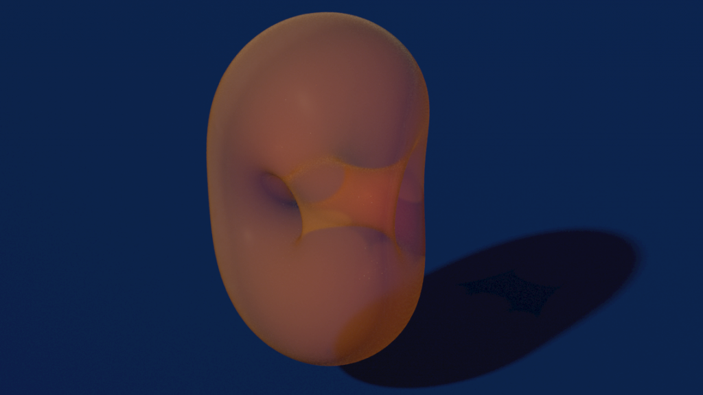
To produce Lawson’s minimal surfaces we need to solve then the Plateau problem for geodesic quadrilaterals \(\square_{k,m}=P_1Q_qP_2Q_2\) in \(\mathbb S^3\), where\[P_1,P_2 \in C_1 = \{(z,w)\in \mathbb S^3 \subset \mathbb C^2 \cong \mathbb R^4 \mid |z| = 1\},\quad \mathrm{dist}(P_1,P_2) = \frac{\pi}{k+1}\]and\[Q_1,Q_2 \in C_2 = \{(z,w)\in \mathbb S^3 \subset \mathbb C^2 \cong \mathbb R^4 \mid |w| = 1\},\quad \mathrm{dist}(Q_1,Q_2) = \frac{\pi}{m+1}\,.\]Let us restrict attention only to the case \(m=1\). In this case \(k\) is just the number of handles—the genus of the surface.
Under the stereographic projection the quadrilateral \(\square_{k,1}\) look as follows
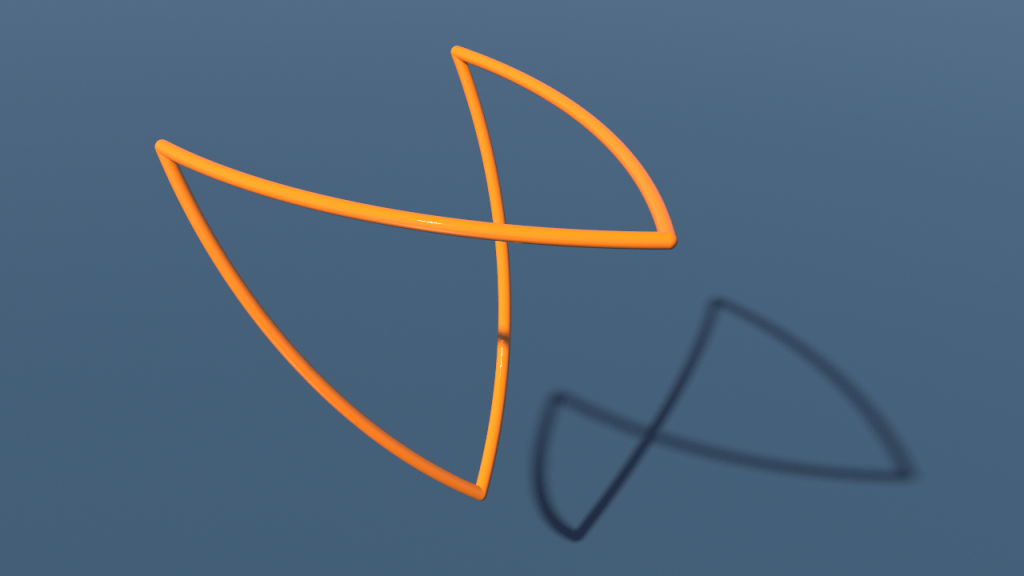
For the figure used the stereographic projection from northpole \(e_4\in \mathbb R^4\) where the square \(\square_{k,1}\) (here \(k=2\)) was sampled by the discrete curve \(\gamma\colon \mathbb Z/4n\mathbb Z \to \mathbb C^2\) with \(4n\) vertices given by\[\gamma_j = \cases{\Bigl(\cos(\tfrac{\pi j}{2n})\mathbf 1,\sin(\tfrac{\pi j}{2n})\mathbf e^{-\tfrac{\pi\mathbf i}{4}}\Bigr) & for \(0\leq j\,\%\,4n<n\) \\\Bigl(\cos(\tfrac{\pi j}{2n})\mathbf e^{\pi\mathbf i – \tfrac{\pi\mathbf i}{k+1}},\sin(\tfrac{\pi j}{2n})\mathbf e^{-\tfrac{\pi\mathbf i}{4}}\Bigr) & for \(n\leq j\,\%\,4n < 2n\) \\\Bigl(\cos(\tfrac{\pi j}{2n})\mathbf e^{\pi\mathbf i – \tfrac{\pi\mathbf i}{k+1}},\sin(\tfrac{\pi j}{2n})\mathbf e^{\tfrac{\pi\mathbf i}{4}}\Bigr) & for \(2n\leq j\,\%\,4n<3n\) \\\Bigl(\cos(\tfrac{\pi j}{2n})\mathbf 1,\sin(\tfrac{\pi j}{2n})\mathbf e^{\tfrac{\pi\mathbf i}{4}}\Bigr) & for \(3n\leq j\,\%\,4n<4n\)}\,.\]In Houdini we can easily implement this formula starting with a circle node with \(4n\) vertices and store the points of \(\square_{k,1}\) as vector4 point attribute p@f using a point wrangle node.
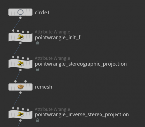
Now given the boundary polygon we want to have a surface \(f\) to start with. Usually we can get such surface using a remesh node. Unfortunately this node only works on point positions in \(\mathbb R^3\). Though it also interpolates the values of p@f which then can be normalized, it turns out to be better to remesh instead the stereographic projection which then can be mapped back to the \(3\)-sphere using the inverse stereographic projection. Here how the network might look at this point:
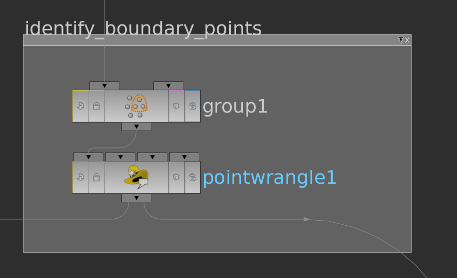
Furthermore we again need to identify interior points. This e.g. can be done by a sequence of group nodes:
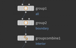
Here the first group node just collects all the points by the base group option. The second only selects boundary vertices, which then are subtracted from the first group using a group combine node.
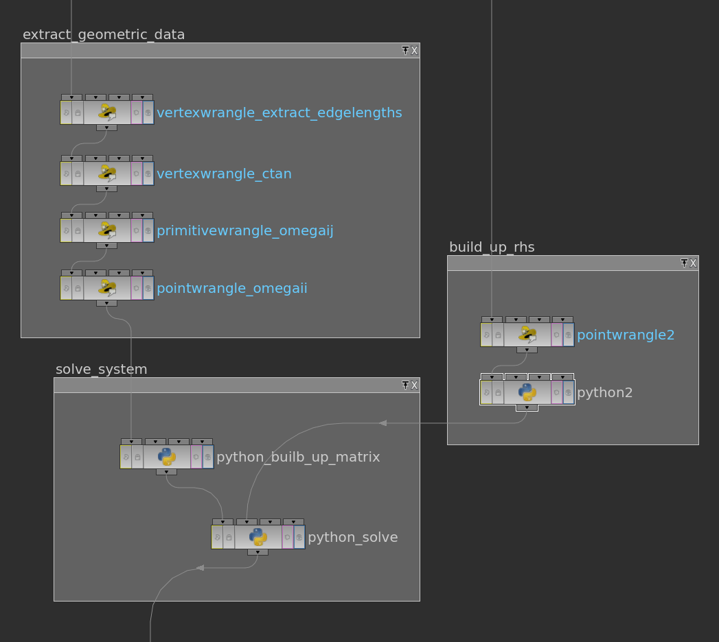
Now we are ready to iterate. This can be done by a loop node as we already used or—if one is interested in the progress of the iteration using a solver node

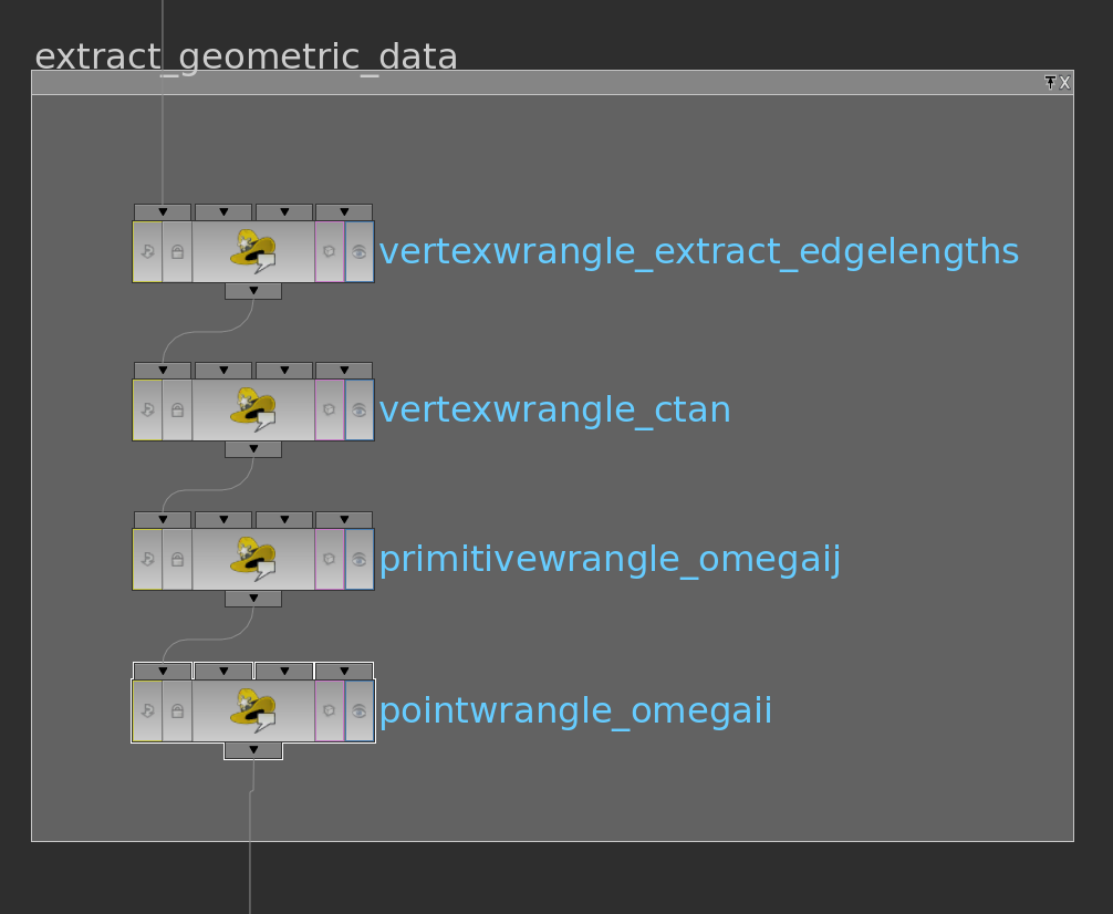
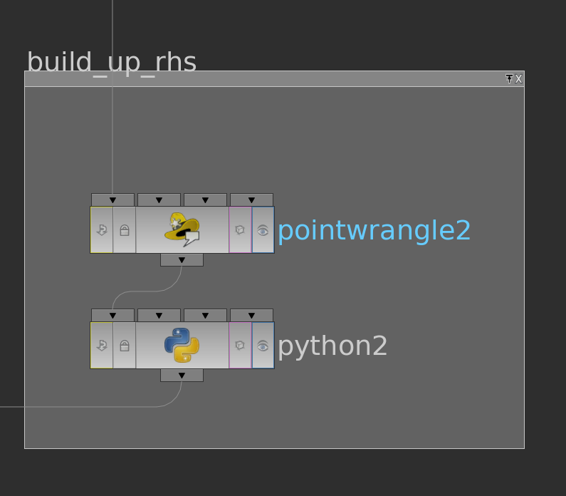
which performs one step per frame when then play button at the lower left corner is hit. The network inside look as follows:
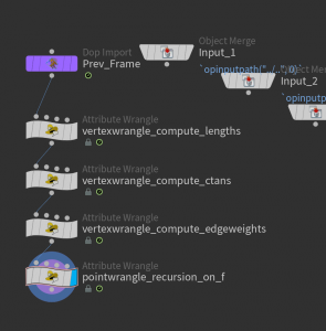
Here the cotangent weight of the current immersion are computed using vertex wrangle nodes. After that we use point wrangle node on the interior point group to perform the iteration on the vector4 attribute p@f. Here a sequence of frames how the results may look like:
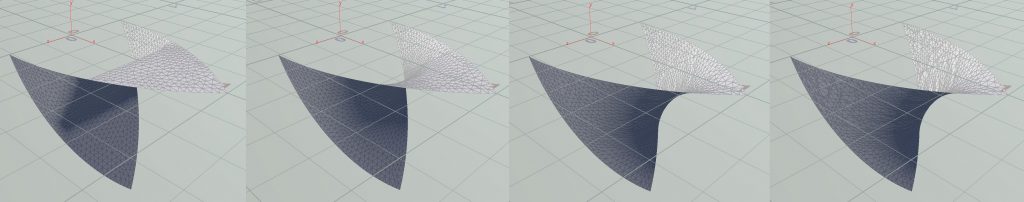
The first picture shows the first frame while the last shows the 2000th.
After we solved the Plateau problem we can rotate and reflect the quadrilateral to form a larger piece. This is done here in a subnetwork which at the end spits out the stereographic projection
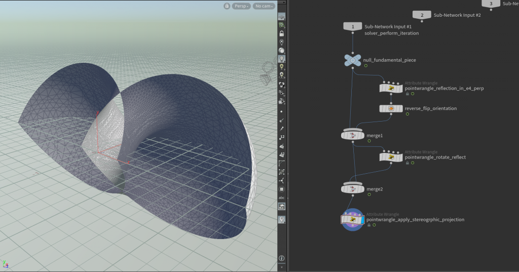
Here the point wrangle node reflect_in_e4_perp multiplies the 4th component of p@f by \(-1\). The second also contains just one line as well
p@f = set(p@f[0],-p@f[1],-p@f[3],p@f[2]);
The resulting patch can then be copied and rotated \((k+1)\)-times around the \(z\)-axis to form the Lawson surface. Using a fuse node we can even turn the patches into a single closed surface which then can be remeshed if needed:
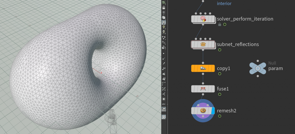
Here you also see a null node to globally store the parameters \(k\) and \(n\).
In particular we are now able to produce closed minimal surfaces in the \(3\)-sphere of arbitrary genus. Here a Lawson surface of genus \(7\):
Homework (due 18 June). Build a network that computes for a given \(k>0\) the corresponding Lawson surface.
Posted in Tutorial
Leave a comment
Tutorial 8: Electric Fields on Surfaces
As described in the lecture a charge distribution \(\rho\colon \mathrm M \to \mathbb R\) in a uniformly conducting surface \(M\) induces an electric field \(E\), which satisfies Gauss’s and Faraday’s law\[\mathrm{div}\,E = \rho, \quad \mathrm{curl}\, E = 0.\]In particular, on a simply connected surface there is an electric potential \(u\colon \mathrm M \to \mathbb R\) such that\[ E =-\mathrm{grad} \,u.\]If we then apply the divergence operator on both sides we find that \(u\) solves the following Poisson problem\[\Delta u = -\rho.\]The potential is determined up to an additive constant thus the field is completely determined by the equation above. Since we have a discrete Laplace operator on a triangulated surface we can easily compute the electric field of a given charge:
- Compute \(\Delta\) and solve for the electric potential \(u\).
- Compute its gradient and set \(E = -\mathrm{grad}\, u\).
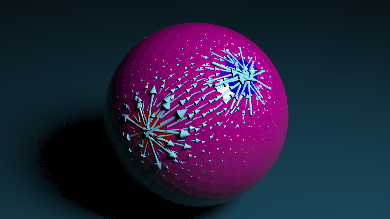
Here the resulting field for a distribution of positive and negative charge on the sphere:
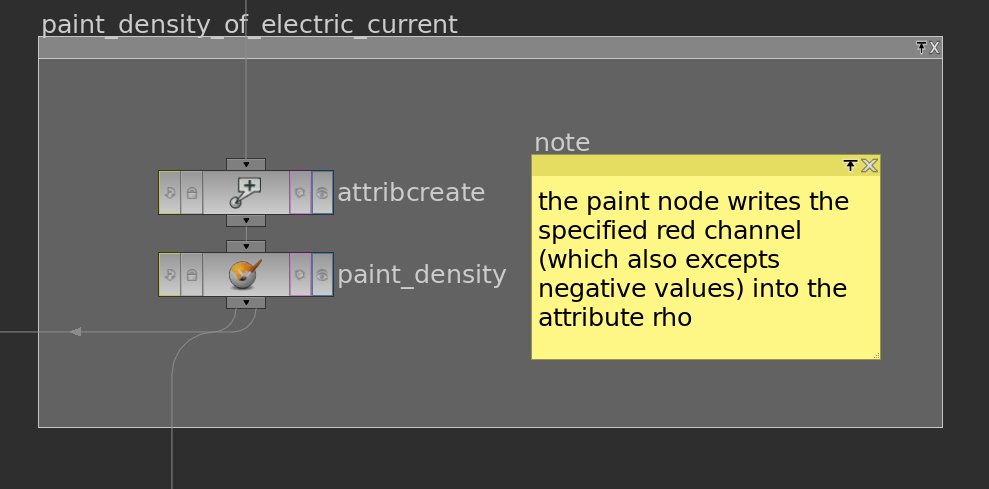
Though there are some issues. First, we need first paint the density \(\rho\) onto \(\mathrm M\). Therefore we can just use a paint node – it has an override color flag where one can specify which attribute to write to.
A bit more serious problem is that not every density distribution leads to a solvable Poisson problem. Let us look a bit closer at this. We know that\[\Delta = A^{-1} L,\]where \(A\) is the mass matrix containing vertex areas and \(L\) contains the cotangent weights – as described in a previous post. We know that \[\mathrm{ker}\, \Delta = \{f\colon V \to \mathbb R \mid f = const\}\]and that \(\Delta\) is self-adjoint with respect to the inner product induced by \(A\) on \(\mathbb R^V\), \(\langle\!\langle f,g\rangle\!\rangle = f^t A g\). In this situation we know from linear algebra that\[\mathbb R^V = \mathrm{im}\, \Delta \oplus_\perp \mathrm{ker}\, \Delta.\]Hence the Poisson equation \(\Delta u = -\rho\) is solvable if and only if \(\rho\) is perpendicular to the constant functions, in other words\[\langle\!\langle \rho , 1 \rangle\!\rangle = \sum_{i\in V} \rho_i A_i =0.\]This is easily achieved by subtracting the mean value of \(\rho\) (orthogonal projection):\[\rho_i \leftarrow \rho_i -\tfrac{ \sum_{k\in V} \rho_k A_k}{\sum_{k\in V} A_k}.\]Then the Poisson equation \(\Delta u = – \rho\) is solvable and defines an electric field.
Actually symmetric systems are also better for the numerics. Thus we solve instead\[L u = – A \rho.\]Since the matrix \(L\) is symmetric we can use the cg-solver which is quite fast and even provides a solution if \(L\) has a non-zero kernel – provided that \(-A\rho\) lies in the image of \(L\).
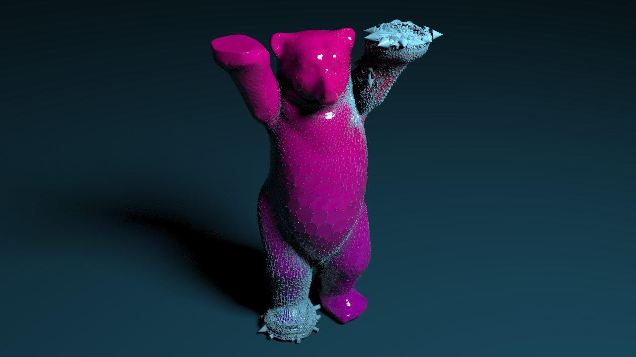
Below the electric potential on the buddy bear where we have placed a positive charge on its left upper paw and a negative charge under its right lower paw.
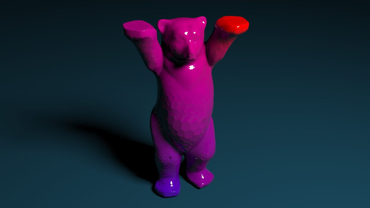
Actually the bear on the picture does not consist of triangles – we used a divide node to visualize the dual cells the piecewise constant functions live on.
The graph of the function \(u\) (which is stored as a point attribute @u) can then be visualized by a polyextrude node. Therefore one selects Individual Elements in the Divide Into field and specifies the attribute u in the Z scale field.
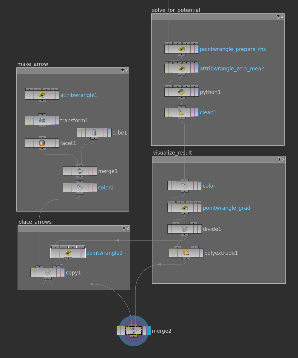
The dual surface also provides a way to visualize the electric field: Once one has computed the gradient (on the primitives of the triangle mesh) the divide node turns it into an attribute at the points of the dual surface (corresponding to the actual triangles). This can then be used to set up attributes @pscale (length of gradient) and @orient (quaternion that rotates say \((1,0,0)\) to the direction of the gradient) and use them in a copy node to place arrows. Reading out the gradient at the vertices of the dual mesh needs a bit care:
vector g  = v@grad;
p@orient = dihedral(set(1,0,0),g);
@pscale = length(g);
Here how the end of the network might look like:
And here the resulting image:
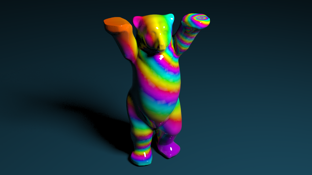
Since the potential varies quite smoothly the coloring from blue (minimum) to red (maximum) does not reveal much of the function. Another way to visualize \(u\) is by a periodic texture. This we can do using the method hsvtorgb, where we can stick in a scaled version of u in the first slot (hue).
Homework (due 11 June). Build a network that allows to specify the charge on a given geometry and computes the corresponding electric field and potential.
Posted in Tutorial
Leave a comment
Tutorial 7: The Discrete Plateau Problem
In the lecture we have defined what we mean by a discrete minimal surface. The goal of this tutorial is to visualize such minimal surfaces.
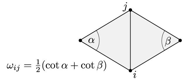
Let \(\mathrm M\) be a discrete surface with boundary and let \(V, E, F\) denote the set of vertices, (unoriented) edges and faces. Once we have a discrete metric, i.e. a map \(\ell \colon E \to (0,\infty)\) such that the triangle inequalities hold,\[\ell_{ij} \leq \ell_{ik}+ \ell_{kj}, \quad \ell_{jk}\leq \ell_{ji} + \ell_{ik},\quad \ell_{ki} \leq \ell_{kj}+ \ell_{ji},\quad \textit{ for each }\sigma = \{i,j,k\},\]we can define the corresponding discrete Dirichlet energy \(E_D^\ell\):\[E_D^\ell (f) = \sum_{ij\in \tilde E} \omega_{ij}^\ell\,(f_j-f_i)^2,\quad \omega^\ell_{ij} = \tfrac{1}{2}(\cot \alpha_{ij} + \cot\beta_{ij}).\]Here \(\tilde E\) denote the positively oriented edges. Certainly the angles and thus the cotangent weights depend on the metric \(\ell\).
In particular, each map \(f\colon \mathrm M \to \mathbb R^3\), which maps thecombinatoric triangles to a non-degenerate triangles in \(\mathbb R^3\), yields an induced discrete metric,\[\ell_{ij} = |p_j – p_i|.\]We have seen in the lecture that a surface is minimal, i.e. a critical point of the area functional under all variations fixing the boundary, if and only if it solves the Dirichlet problem (with respect to its induced metric): For each interior vertex \(i\in\mathring V\) we have\[-\tfrac{1}{2}\sum_{\{i,j\}\in E}\,\omega_{ij}^\ell f_i +\tfrac{1}{2}\sum_{\{i,j\}\in E}\,\omega_{ij}^\ell f_j = 0,\]where \(\ell\) denotes the metric induced by \(f\).
Unfortunately, unlike the Dirichlet problem, this is a non-linear problem—the cotangent weights depend on \(\ell\) in a complicated way. Though, fortunately, we can solve it in many cases by iteratively solving a Dirichlet problem (here a paper that describes this). Since we know how to solve the Dirichlet problem we can implement this method without any effort.
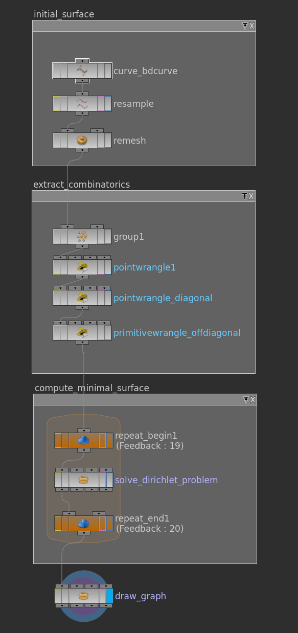
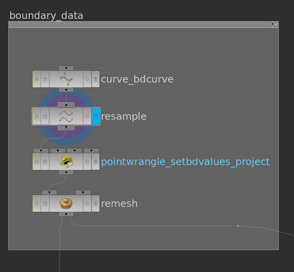
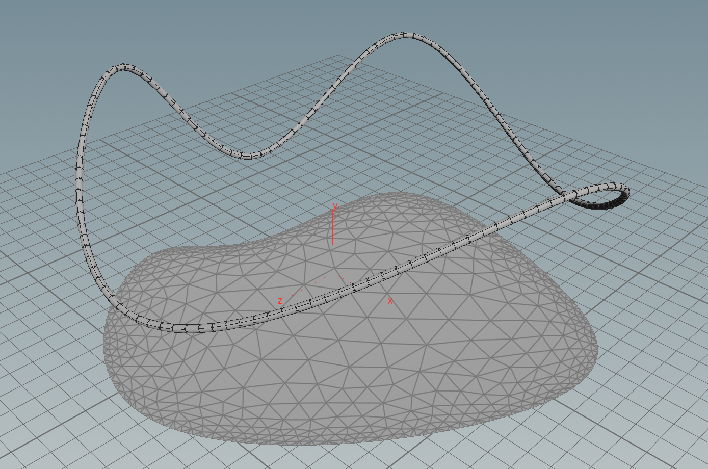
The network above visualizes Plateau’s problem: Given a space curve \(\gamma\) compute a minimal disk with boundary \(\gamma\). Actually this corresponds to a soap film spanned into a wire.

In the discrete setup we start with some discrete space, say generated by a curve node (probably followed by a resample node), which we then stick into a remesh node to get a reasonably triangulated disk spanned in. Then we can apply the iteration to this input. Below one possible result:
For rendering we used here the following texture in the mantra surface material. To generate texture coordinates one can use the nodes uvunwrap or uvtexture.
The algorithm is not restricted to disks. We can stick in any surface we want. Another nice example is e.g. obtained by starting with a cylinder of revolution. Here the minimal surface becomes a part of a catenoid or, if the cylinder’s height becomes to large, it degenerates to a pair of flat disks (connected by a straight line). In the picture below the last two circles are already too far apart – the surface starts to splits into two parts.
As a last example we can start with the unit sphere into which we cut several holes. If we want nice symmetries we could use a platonic solid node to copy smaller spheres to the vertex positions of e.g. an octahedron. The area enclosed by the smaller spheres we then subtract from the unit sphere with help of a cookie node. If we run then the algorithm on this input we end up with nice symmetric minimal surface. For a certain radius of the holes the surface is close to the Schwarz P surface.
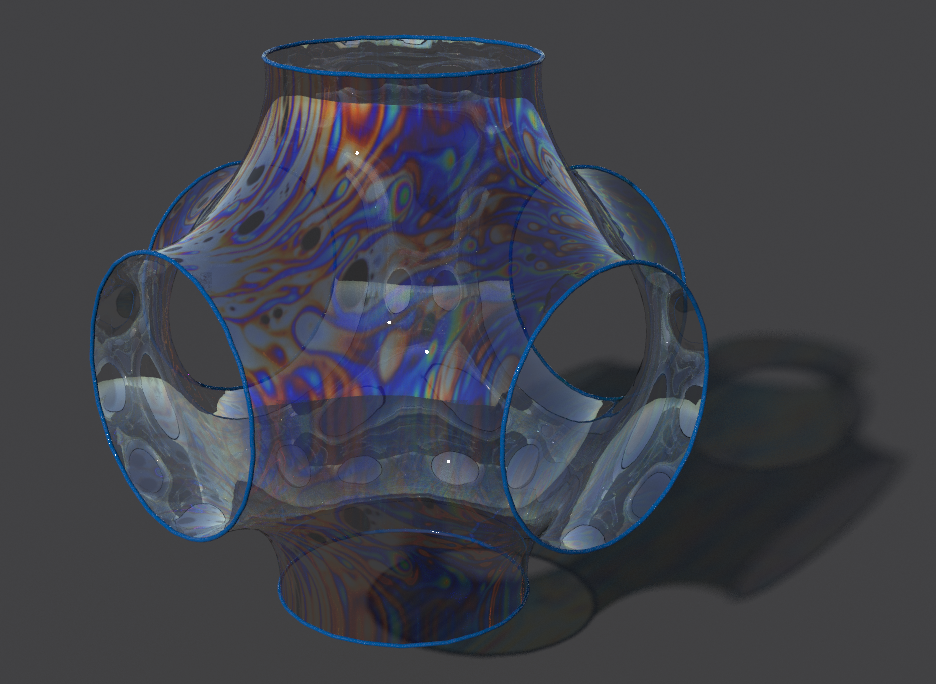
Again one can observe the same effect as for the cylinder—if the holes get to small the minimal surface degenerates to several spheres connected to the origin.
Homework (due 4 June). Build a network that computes from a given discrete surface with boundary a minimal surface with the same boundary. Use this network to solve Plateau’s problem and to compute symmetric minimal surface from a sphere with holes as described above.
Posted in Tutorial
Leave a comment
Tutorial 6: The Dirichet Problem
In the lecture we saw that the Dirichlet energy has a unique minimizer among all functions with prescribed boundary values. In this tutorial we want to visualize these minimizers in the discrete setting.
Let \(\mathrm M\subset \mathbb R^2\) be a triangulated surface with boundary \(\partial \mathrm M\) and let \(V\), \(E\) and \(F\) denote the set of vertices, edges and triangles of the underlying simplicial complex \(\Sigma\). Further, let \(p_i\in \mathbb R^2\) denote the position of the vertex \(i\in V\).
To each discrete function \(f\in\mathbb R^V\) we assigned a corresponding piecewise affine function \(\hat f=\sum_{i\in V}f_i\phi_i\). Here \(\phi_i\) denotes the hat function corresponding to the vertex \(i\), i.e. \(\phi_i\) is the unique piecewise affine function such that \(\phi_i(p_j) = \delta_{ij}\).
Further we have computed the Dirichlet energy of an affine function \(\hat f\) on a single triangle: If \(T_\sigma \subset \mathbb R^2\) denotes the triangle corresponding to \(\sigma=\{i,j,k\}\in F\) and \(\alpha_{jk}^i\) denotes the interior angle in \(T_\sigma\) at the vertex \(i\), then\[ \int_{T_\sigma} \bigl|\mathrm{grad}\, \hat f\bigr|^2 = \tfrac{1}{2}\bigl(\cot \alpha_{jk}^i\,(f_j – f_k)^2 +\cot \alpha_{ki}^j\,(f_k – f_i)^2 +\cot \alpha_{ij}^k\, (f_i – f_j)^2\bigr).\]The Dirichlet energy of a discrete function \(f\in \mathbb R^V\) is then defined as the Dirichlet energy of the corresponding piecewise affine function \(\hat f\):\begin{align}2\,E_D(f) & = \sum_{\sigma \in \Sigma} \int_{T_\sigma} \bigl|\mathrm{grad}\, \hat f\bigr|^2 =\sum_{\{i,j,k\} \in F} \tfrac{1}{2}\bigl(\cot \alpha_{jk}^i (f_j – f_k)^2 +\cot \alpha_{ki}^j (f_k – f_i)^2 +\cot \alpha_{ij}^k (f_i – f_j)^2\bigr)\\&=\sum_{\{i,j\} \in E} \sum_{\{i,j,k\}\in F}\tfrac{1}{2}\cot \alpha_k^{ij} (f_i – f_j)^2.\end{align}As a quadratic form the Dirichlet energy has a corresponding symmetric bilinear form: Let\[\omega_{ij} = \tfrac{1}{2}\sum_{\{i,j,k\}\in F}\cot\alpha_{ij}^k\] and define \(\mathbf L\) by \[\mathbf L_{ij} = \cases{-\sum_{{i,k}\in E}\omega_{ik},& if \(i=j\),\\\omega_{ij},& if \(\{i,j\}\in E\)\\ 0, & else,}\]then\[E_D(f) = -\tfrac{1}{2}\,f^T \mathbf L \, f.\]Note, that on a surface each edge is contained in exactly one or two triangles. Thus the weights \(\omega_{ij}\) are sums of only one or two cotangents as illustrated in the picture below for the case of an inner edge.
Now let \(\mathring V\) denote the set of interior vertices and set \(V_{bd}: = V\setminus \mathring V\). To each \(g\colon V_{bd} \to \mathbb R\) we define an affine space\[W_g := \bigl\{f\in \mathbb R^V \mid \left.f\right|_{V_{bd}}= g\bigr\}.\]Given \(g\) we are looking for a critical points of the restriction \(E_D\colon W_g \to \mathbb R\). Therefore we compute the derivative of \(E_D\): Let \(f\in W_g\) and let \(f_t\) be a curve in \(W_g\) through \(f\) with \(X = \left.\tfrac{d}{dt}\right|_{t=0}\,f_t\). Then we get\[d_f E_D\,(X) =\left.\tfrac{d}{dt}\right|_{t=0} E_D(f_t) = -\tfrac{1}{2}\left.\tfrac{d}{dt}\right|_{t=0}\, (f_t^T \mathbf L\, f_t) =-\tfrac{1}{2}f^T \mathbf L\, X -\tfrac{1}{2}X^T \mathbf L\, f= -X^T\mathbf L\,f.\]Since \(f_t \in W_g\) for all \(t\) we obtain that \(X\in W_0\), i.e. \(\left.X\right|_{V_{bd}} = 0\). Conversely each \(X\in W_0\) yields a curve in \(W_g\) through \(f\). Thus \(f\) is a critical point of \(E_D\) if and only if the entries of \(\mathbf L\,f\) corresponding to interior vertices vanish: For each vertex \(i\in \mathring V\) we have \[\sum_{\{i,j\}\in E} \omega_{ij}f_i-\sum_{\{i,j\}\in E} \omega_{ij}f_j = \sum_{\{i,j\}\in E} \omega_{ij}(f_i- f_j) = 0.\]Since \(E_D\) is convex there is always a global minimum and thus there is always a solution. As in the smooth case the minimizer is unique.
To summarize: Given any function \(g\colon V_{bd}\to \mathbb R\), the unique minimizer \(f\in W_g\) of the Dirichlet energy is the solution of the following linear system\[\cases{\sum_{\{i,j\}\in E} \omega_{ij}(f_i- f_j) = 0, & for each \(i\in \mathring V\),\\f_i = g_i, & for each \(i\in V_{bd}\).}\]
Now we want to build up a network that computes the minimizer for given a function given on the boundary of a surface in \(\mathbb R^2\).
First we need to specify a surface in \(\mathbb R^2\) and a function \(g\) on its boundary. One possible way to do this is to use a space curve: First we draw with a curve node a space curve and probably resample it. Then we use the say y-component as the function \(g\) on the boundary and project it to a polygon in the plane xz-plane and remesh it. Here the network
The pointwrangle node contains the following 3 lines of code:
f@g =  @P.y;
v@P.y = 0;
f@f;
Then we have a triangulated surface in the plane and a graph over its boundary (the curve we started with).
Now we want to build up the matrix \(\mathbf A\) of the linear system. To solve the system we will use scipy. Though, for performance reasons, we will do as much as we can in VEX, which is much faster than python. In particular we will avoid python loops when filling the matrix.
We will use a compressed sparse row matrix (scipy.sparse.csr_matrix). The constructor needs 3 arrays of equal length – two integer arrays (rows,colums) specifying the position of non-zero entries and a double array that specifies the non-zero entries – and two integers that specify the format of the matrix.
The non-zero entries in \(\mathbf A\) are exactly the diagonal entries \(\mathbf A_{ii}\) and the off-diagonal entries \(\mathbf A_{ij}\) that belong to oriented edges \(ij\) of the surface. Accessing Houdini point attributes and Houdini primitive attributes in python is fast, but unfortunately that’s not the case for the Houdini vertex attributes. Fortunately, we can store the vertex attribute in vectors sitting on primitives: For a surface the Houdini vertices of the primitives are one-to-one with its halfedges – each vertex is the start vertex of a halfedge in the boundary of the Houdini primitive.
By this observation above we can get a complete array of non-zero value indices as follows: we can store an attribute i@id = @ptnum (@ptnum itself is not accessible from python) on points and two attributes v@start and v@end (encoding row and column resp.) on Houdini primitive that contain for each edge in the primitive (starting from primhedge(geo,@primnum)) the point number of the source point (@start) and destination point (@end) of the current edge in the Houndini primitive.
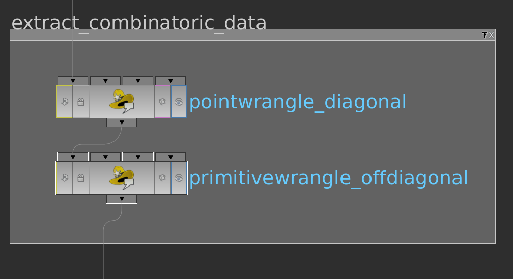
Here the VEX code of the primitivewrangle node:
int he = primhedge(0,@primnum);

int p1 = hedge_srcpoint(0,he);
int p2 = hedge_dstpoint(0,he);
int p3 = hedge_presrcpoint(0,he);

v@start = set(p1,p2,p3);
v@end = set(p2,p3,p1);
The pointwrangle node just contains one line (i@id = @ptnum;).
Before we can finally start to compute the cotangent weights and write the matrix entries to attributes we still need one more information – whether a point lies on the boundary or not. This we can do e.g. as follows:
The group node has in its edge tab a toggle to detect ‘unshared edges’, i.e. edge which appear in only one triangle. With this we build a group boundary over whose points we then run with a pointwrangle node setting an attribute i@bd = 1 (the other points then have @bd = 0 per default).
Now let us start to compute the matrix entries. We will do this here in several steps.
Here VEX code of the wrangle nodes in their order:
int he = vertexhedge(0,@vtxnum);
vector P = attrib(0,'point','P',hedge_srcpoint(0,he));
vector Q = attrib(0,'point','P',hedge_dstpoint(0,he));
f@edgelength = length(P-Q);
float getCosineAlpha(float a,b,c) {
    float d = b * b + c * c - a * a;
    float e = 2 * b * c;
    return  d / e;
}

float getCotangentAlpha(float a,b,c) {
    float cosalpha = getCosineAlpha(a, b, c);
    float d = 1 - cosalpha * cosalpha;
    return cosalpha / sqrt(d);
}

int this = @vtxnum;
int he = vertexhedge(0,this);
int next = hedge_dstvertex(0,he);
int prev = hedge_presrcvertex(0,he);

float a = attrib(0,'vertex','edgelength',this);
float b = attrib(0,'vertex','edgelength',next);
float c = attrib(0,'vertex','edgelength',prev);

f@ctan = getCotangentAlpha(a,b,c);
float getCotangentWeight(int geo; int he){
    int opphe = hedge_nextequiv(geo,he);
    int v1 = hedge_srcvertex(geo,he);
    int v2 = hedge_srcvertex(geo,opphe);
    int bd1 = attrib(geo,'point','bd',vertexpoint(0,v1));
    int bd2 = attrib(geo,'point','bd',vertexpoint(0,v2));
    if(bd1 == 1){
        return 0;
    }else{
        // the startvertex determines the row the weight finally ends up
        // for boundary vertices all row entries up to the diagonal
        // entry shall vanish
        float cotanleft = attrib(geo,'vertex','ctan',v1);
        float cotanright = attrib(geo,'vertex','ctan',v2);
        return -(cotanleft+cotanright)/2.;

    }
}

int he = primhedge(0,@primnum);
float c1 = getCotangentWeight(0,he);
he = hedge_next(0,he);
float c2 = getCotangentWeight(0,he);
he = hedge_next(0,he);
float c3 = getCotangentWeight(0,he);
v@omega = set(c1,c2,c3);
if(attrib(0,'point','bd',@ptnum) == 1){
    // diagonal entries corresponding to boundary values shall be 1
    f@omega = 1.;
}else{
    // else summ the values on the vertex/edge star
    int he0 = pointhedge(0,@ptnum);
    int he = he0;
    int opphe;
    f@omega = 0;
    do{
        opphe = hedge_nextequiv(0,he);
        // weights of Laplacian
        @omega += attrib(0,'vertex','ctan',hedge_srcvertex(0,he))/2.;
        @omega += attrib(0,'vertex','ctan',hedge_srcvertex(0,opphe))/2.;
        he = pointhedgenext(0,he);
    }while(he!=he0 && he!=-1);
}
Now that we have set up the values we can build up the matrix in a python node: The attributes can read out of the Houdini geometry (geo) using methods as pointIntAttribValues(“attributename”) or primFloatAttribValues(“attributename”). The arrays are concatenated by numpy.append and then handed over to the csr_matrix-constructor. To access the matrix in the next node we can store it as cachedUserData in the node (compare the code below).
from scipy.sparse import csr_matrix
import numpy as np
import math

### get geometry

node = hou.pwd()
geo = node.geometry()

n = len(geo.points())

### get point and prim attributes

pointid = np.array(geo.pointIntAttribValues("id"))
start = np.array(geo.primIntAttribValues("start"))
end = np.array(geo.primIntAttribValues("end"))

omegaii = np.array(geo.pointFloatAttribValues("omega"))
omegaij = np.array(geo.primFloatAttribValues("omega"))

### prepare matrix

# non-zero matrix elements:
# first the diagonal entries, then the entries corresponding to half edges
rowids = np.append(pointid,start)
colids = np.append(pointid,end)

# values of Laplacian and mass corresponding to (row,col) specified above
valueslaplacian = np.append(omegaii,omegaij)

### initialize matrices
laplace = csr_matrix((valueslaplacian,(rowids,colids)),(n,n))

# set cached user data
node.setCachedUserData("laplace",laplace)
We still need to prepare the right hand side of the system. Therefore we extend the function \(g\) defined on the boundary vertices to the interior vertices by zero (pointwrangle node) and store it as cachedUserData as well (python node).
Here the corresponding code
if(@bd == 0) @g= 0;
import numpy

node = hou.pwd()
g = numpy.array(node.geometry().pointFloatAttribValues("g"))
node.setCachedUserData("g", g)
Now we stick both python node – the one in which we stored the matrix and the one in which we stored the right hand side – into another one where we finally solve the linear system.
The cached user data can be accessed by its name. The easiest way to solve the system is to use scipy.sparse.linalg.spsolve. After that the solution is stored as a point attribute. Below the corresponding python code:
from scipy.sparse.linalg import spsolve
import numpy

node = hou.pwd()
geo = node.geometry()

laplace = node.inputs()[0].cachedUserData("laplace")
g = node.inputs()[1].cachedUserData("g")

f = spsolve(laplace,g)

geo.setPointFloatAttribValuesFromString("f",f.astype(numpy.float32))
Though this can be speeded up when rewriting the system as an inhomogeneous symmetric system, which can then be solved by scipy.sparse.linalg.cg. Here the alternative code:
from scipy.sparse.linalg import cg
import numpy as np

node = hou.pwd()
geo = node.geometry()

isbd = np.array(geo.pointIntAttribValues("bd"),dtype="bool")
isin = np.logical_not(isbd)

laplace = node.inputs()[0].cachedUserData("laplace")
g = node.inputs()[1].cachedUserData("g")

laplaceI = laplace[isin,:]
laplaceII = laplaceI[:,isin]
laplaceIB = laplaceI[:,isbd]

gb = g[isbd]

x,tmp = cg(laplaceII,-laplaceIB.dot(gb))

f = g
f[isin] = x

geo.setPointFloatAttribValuesFromString("f",f.astype(np.float32))
Now we are back in VEX land and we can finally draw the graph of the solution:
Homework (due 28 May). Build a network which allows to prescribe boundary values and then computes the corresponding minimizer of the Dirichlet energy.
Posted in Tutorial
Leave a comment
Plateau problem
Let $\Sigma = (V,E,F)$ be a triangulated surface (with boundary). A realization of the surface in $\mathbb{R}^3$ is given by a map $p:V \rightarrow \mathbb{R}^3$ such that $p_i,p_j,p_k$ form a non degenerated triangle in $\mathbb{R}^3$ for all $\{i,j,k\} \in \Sigma$, (i.e. $p_i,p_j,p_k$ do not lie on a line). Some problems, like the plateau problem do not depend on the position of the vertices in the space, but only on the length of the edges:
\[l_{ij} = l_{ji} = |e_{ji}| \quad \quad {i,j} \in E. \]
If we have a realization of the surface in $\mathbb{R}^3$ there holds: $l_{ij}= l_{ji}=|p_i-p_j|$ and the edge length’s satisfy the triangle inequalities:
\[\mbox{For } \{i,j,k\} \in F \Rightarrow \left\{ \begin{matrix} l_{ij} < l_{jk} + l_{ki}, \\ l_{ki} < l_{ij} + l_{jk}, \\ l_{jk} < l_{ki} + l_{ij}. \end{matrix} \right .\]
Definition: A metric on a triangulated surface assigns a length to each oriented edge such that the triangle inequalities are satisfied.
 Note that every realization $p:V \rightarrow \mathbb{R}^3$ induces a metric on the underlying triangulated surface. On the other hand a triangulated surface with metric has several realization in $\mathbb{R}^3$, such that the metrics coincide. On a triangulated surface with metric every triangle has the structure of an euclidean triangle in $\mathbb{R}^2$, that allows us to interpolate $f:V\rightarrow \mathbb{R}$ to a piecewise affine function $\tilde{f}: C\left( \Sigma\right) \rightarrow \mathbb{R}$ and define the Dirichlet energy $E_D(f)$ as in the last lectures.
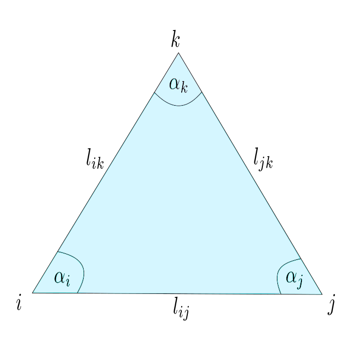
In particular, we can define angles and area using the cosine theorem:
\[\cos(\alpha_i) = \frac{l_{jk}^2-l_{ji}^2-l_{ki}^2}{2l_{ki}l_{ij}}\]
By the triangle inequalities we obtain that $0 < \gamma <\pi$ and the angles are well defined. With $\sin(\alpha_i) = \sqrt{1-\cos(\alpha_i)^2}$ we can define the cotangents weights and the area of the triangle $\sigma = \{i,j,k\}$ :
\[A_{\sigma} = \frac{1}{2} \sin{(\alpha_i})l_{ij} l_{ki}.\]
For a realization $p$ of $\Sigma$ with vertex positions $p_i,p_j,p_k$ and edges $e_{ij} = p_j-p_i, \ldots $ we obtain for $\sigma = \{i,j,k\} \in F$:
\[A_{\sigma}(p) = \frac{1}{2}\left| (p_j-p_i) \times (p_k-p_i) \right| = \frac{1}{2}\left| e_{ij} \times e_{ik}\right| = \frac{1}{2} \sin{(\alpha_i})\underbrace{|e_{ij}|}_{ =l_{ij}} \underbrace{|e_{ki}|}_{=l_{ki}},\]
and the total area is give by:
\[A (p) = \sum_{\sigma \in F} A_{\sigma}(p).\]
Definition: The following problem is the Plateau problem: Let $\Sigma$ be a triangulated surface with boundary and $q: V^{\partial} \rightarrow \mathbb{R}^3 $ a prescribed function. We are looking for a realization $p:V \rightarrow \mathbb{R}^3$ of $\Sigma$ such that:
1. $\left. p \right|_{V^{\partial}} = q,$
2. $ p$ has the smallest area among all realizations $ \tilde{p}$ of $\Sigma$, with $ \left. \tilde{p} \right|_{V^{\partial}} = q$.
In order to be able to solve the Plateau problem we have to consider variations of $p$:
Definition: A variation of $p$ with constant boundary assigns to each vertex $i \in V$ a curve $ t \mapsto p_i(t), $ $ t \in (- \epsilon ,\epsilon) ,$ such that:
1. $p_i(0) = p_i $ for all $i \in V.$
2. $p_j(t) = q_j $ for all $ t \in (- \epsilon ,\epsilon)$ if $j \in V^{\partial}$.
Definition: $p$ is called a minimal surface if it is a critical point of the area functional, i.e. :
\[\left. \frac{\partial}{\partial t} \right|_{t=0} A \left(p(t) \right) = 0,\]
for all variations of $p$ with constant boundary.
Lemma: $p$ is a minimal surface if and only if For each $i \in \overset{\circ}{V}$ and each curve $ t \mapsto p_i(t), $ $ t \in (- \epsilon ,\epsilon) $ we have:
\[\left. \frac{\partial}{\partial t} \right|_{t=0} A \left(p_i(t) \right) = \left. \frac{\partial}{\partial t} \right|_{t=0} \sum_{\sigma \in F \, \vert \, i \in \sigma} A_{\sigma} \left(p_i(t) \right) = 0.\]
I.e. $p$ is a critical point of the area functional with respect to all variations with constant boundary, if and only if it is a critical point for all those variations that only move one interior vertex.
Proof: $”\Rightarrow”:$ clear.
$”\Leftarrow:”$ Similar to the following fact from analysis:
All directional derivatives of a function $f: U \rightarrow \mathbb{R}, \quad U \subset \mathbb{R}^n$ vanish at $p \in U$ if and only if all partial derivatives of $f$ vanish at $p$.
$\square$
Theorem: $p$ is a minimal surface if and only if all tree components of $p$ are discrete harmonic functions with respect to the metric induced on $\Sigma$ by $p$.
Proof: 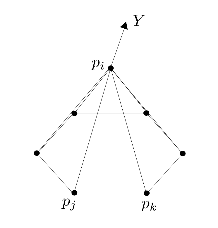 Fix $i \in \overset{\circ}{V}$ and let $ t \mapsto p_i(t), $ $ t \in (- \epsilon ,\epsilon) $ be a variation, that only moves $p_i$ and $Y:= p_i'(o). $ Further we define $\hat{F} := \left\{ \{i,j,k\} \in F \big \vert \mbox{ positive oriented} \right\}$ to be the set of positive oriented triangles that contain the vertex $i$. We have to show that there holds:
\begin{align}0=\left. \frac{\partial}{\partial t} \right|_{t=0} A \left(p_i(t) \right) &= \left. \frac{\partial}{\partial t} \right|_{t=0} \sum_{\{i,j,k\} \in \hat{F}} \left| (p_j-p_i(t)) \times (p_k-p_i(t))\right| \\&= \left. \frac{\partial}{\partial t} \right|_{t=0} \sum_{\{i,j,k\} \in \hat{F}} \left| e_{ij}(t) \times e_{ik}(t) \right|.\end{align}
Before we start with the proof remember these identities from analysis$\backslash$linear algebra
1. For a function $t\rightarrow v(t) \in \mathbb{R}^3$ there holds:
\begin{align} |v|’=\frac{\langle v, v’ \rangle}{|v|} \end{align}
2. For $a,b,c,d \in \mathbb{R}^3$ we have:
\begin{align} \langle a\times b, c \times d \rangle = \det \left( \begin{matrix} \langle a,c \rangle & \langle a,d \rangle \\ \langle b,c \rangle\ &\langle b,d \rangle\ \end{matrix} \right) = \langle a,c \rangle\langle b,d \rangle-\langle a,d \rangle\langle b,c \rangle.\end{align}
With $e_{i,j} = p_j-p_i$ we get $\dot{e_{ij}}=-Y$ and can compute now the variation of the area functional:
\begin{align*} \left. \frac{\partial}{\partial t} \right|_{t=0} &A \left(p_i(t) \right) = \frac{1}{2} \sum_{\{i,j,k\} \in \hat{F}} \frac{\langle e_{ij} \times e_{ik} , -Y \times e_{ik} – e_{ij} \times Y \rangle}{|e_{ij} \times e_{jk}|} \\ &= \sum_{\{i,j,k\} \in \hat{F}} \frac{-\langle e_{ij} ,Y\rangle |e_{ik}|^2 + \langle e_{ik},Y\rangle \langle e_{ij},e_{ik} \rangle -\langle e_{ik} ,Y\rangle |e_{ij}|^2 + \langle e_{ij},Y\rangle \langle e_{ij},e_{ik} \rangle}{2|e_{ij} \times e_{jk}|} \\ &= \bigl\langle Y ,\sum_{\{i,j,k\} \in \hat{F}} \frac{-e_{ij}|e_{ik}|^2-e_{ik}|e_{ij}|^2 + \langle e_{ij},e_{ik} \rangle (e_{ij} + e_{ik})}{2|e_{ij} \times e_{jk}|}\bigr\rangle \\&= \bigl\langle Y ,\sum_{\{i,j,k\} \in \hat{F}} \frac{\left( -\langle e_{ik},e_{ik} \rangle + \langle e_{ij},e_{ik} \rangle\right) e_{ij}+\left( -\langle e_{ij},e_{ij} \rangle + \langle e_{ij},e_{ik} \rangle\right) e_{ik}}{2|e_{ij} \times e_{jk}|} \bigr\rangle.\end{align*}
With \[-\langle e_{ik},e_{ik} \rangle + \langle e_{ij},e_{ik} \rangle = \langle e_{ik},e_{ij} -e_{ik}\rangle =\langle e_{ik},e_{kj} \rangle, \]
and
\[-\langle e_{ij},e_{ij} \rangle + \langle e_{ij},e_{ik} \rangle = \langle e_{ij},e_{ik} -e_{ij}\rangle = \langle e_{ij},e_{jk} \rangle,\]
We have:
\[ \left. \frac{\partial}{\partial t} \right|_{t=0} A \left(p_i(t) \right) = \bigl\langle Y ,\sum_{\{i,j,k\} \in \hat{F}} \left( \frac{ \langle e_{ik},e_{kj} \rangle e_{ij}}{2|e_{ij} \times e_{jk}|} \right) + \sum_{\{i,j,k\} \in \hat{F}} \left( \frac{\langle e_{ij},e_{jk} \rangle e_{ik}}{2|e_{ij} \times e_{jk}|} \right) \bigr\rangle. \]
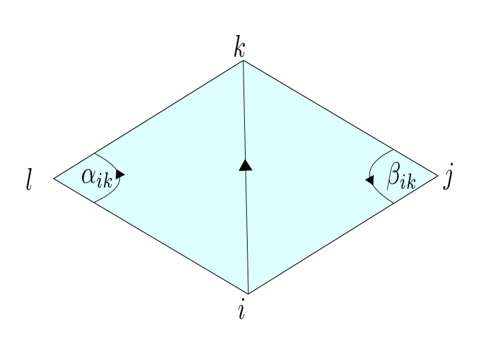
In an earlier lecture we showed that: $\cot(\beta_{ik}) = \frac{\langle -e_{ij},e_{jk}\rangle }{|e_{ij} \times e_{jk}|} $ and $ \cot(\alpha_{ik}) = \frac{\langle e_{il},e_{kl}\rangle }{|e_{ik} \times e_{il}|}. $
With an index shift in the first sum $(i,j,k) \rightarrow (i,k,l)$ we have now : \begin{align*} \left. \frac{\partial}{\partial t} \right|_{t=0} A \left(p_i(t) \right) & = \bigl\langle Y ,-\sum_{\{i,j,k\} \in \hat{F}} \frac{1}{2}\bigl( \cot(\beta_{ik}) + \cot(\alpha_{ik}) \bigr) e_{ik} \bigr\rangle \\ & = \bigl\langle Y , -\sum_{\{i,k\} \in \hat{E}} \frac{1}{2} \bigl( \cot(\beta_{ik}) + \cot(\alpha_{ik}) \bigr) (p_k – p_i) \bigr\rangle. \end{align*}
Since this has to hold for all variations $Y$ of $p_i$ and for all $i \in \overset{\circ}{V} $we finally get:
\[ \left. \frac{\partial}{\partial t} \right|_{t=0} A \left(p(t) \right) =0 \Leftrightarrow \sum_{\{i,k\} \in \hat{E}} \frac{1}{2} \bigl( \cot(\beta_{ik}) + \cot(\alpha_{ik}) \bigr) (p_k – p_i)=0 \quad \forall i \in \overset{\circ}{V}. \]
This means $p$ is an minimal surface if and only if all components of $p$ are harmonic with respect to the metric on $\Sigma$ induced by $p$.
$\square$
Posted in Lecture
Leave a comment