As described in the lecture a charge distribution \(\rho\colon \mathrm M \to \mathbb R\) in a uniformly conducting surface \(M\) induces an electric field \(E\), which satisfies Gauss’s and Faraday’s law\[\mathrm{div}\,E = \rho, \quad \mathrm{curl}\, E = 0.\]In particular, on a simply connected surface there is an electric potential \(u\colon \mathrm M \to \mathbb R\) such that\[ E =-\mathrm{grad} \,u.\]If we then apply the divergence operator on both sides we find that \(u\) solves the following Poisson problem\[\Delta u = -\rho.\]The potential is determined up to an additive constant thus the field is completely determined by the equation above. Since we have a discrete Laplace operator on a triangulated surface we can easily compute the electric field of a given charge:
- Compute \(\Delta\) and solve for the electric potential \(u\).
- Compute its gradient and set \(E = -\mathrm{grad}\, u\).
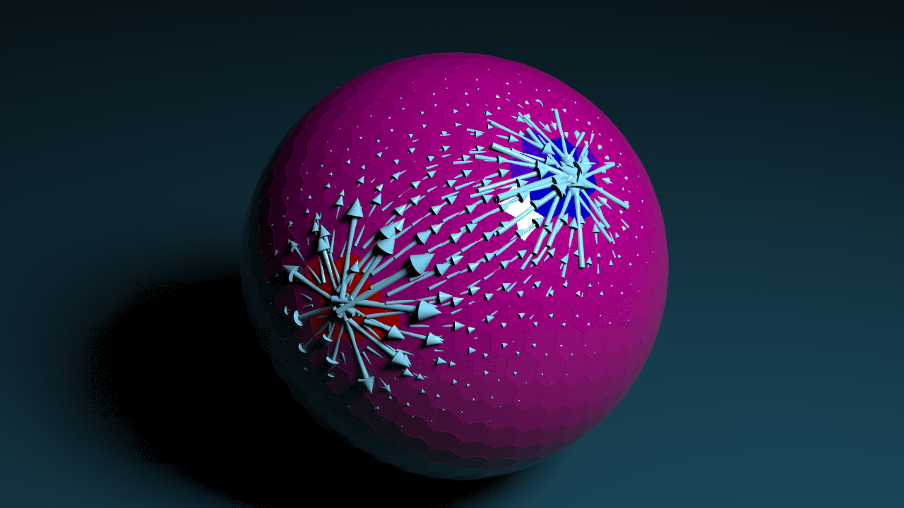
Here the resulting field for a distribution of positive and negative charge on the sphere:
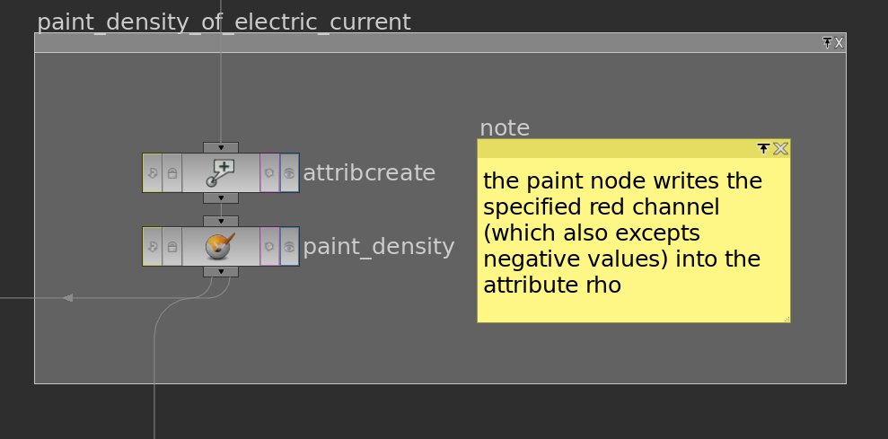
Though there are some issues. First, we need first paint the density \(\rho\) onto \(\mathrm M\). Therefore we can just use a paint node – it has an override color flag where one can specify which attribute to write to.
A bit more serious problem is that not every density distribution leads to a solvable Poisson problem. Let us look a bit closer at this. We know that\[\Delta = A^{-1} L,\]where \(A\) is the mass matrix containing vertex areas and \(L\) contains the cotangent weights – as described in a previous post. We know that \[\mathrm{ker}\, \Delta = \{f\colon V \to \mathbb R \mid f = const\}\]and that \(\Delta\) is self-adjoint with respect to the inner product induced by \(A\) on \(\mathbb R^V\), \(\langle\!\langle f,g\rangle\!\rangle = f^t A g\). In this situation we know from linear algebra that\[\mathbb R^V = \mathrm{im}\, \Delta \oplus_\perp \mathrm{ker}\, \Delta.\]Hence the Poisson equation \(\Delta u = -\rho\) is solvable if and only if \(\rho\) is perpendicular to the constant functions, in other words\[\langle\!\langle \rho , 1 \rangle\!\rangle = \sum_{i\in V} \rho_i A_i =0.\]This is easily achieved by subtracting the mean value of \(\rho\) (orthogonal projection):\[\rho_i \leftarrow \rho_i -\tfrac{ \sum_{k\in V} \rho_k A_k}{\sum_{k\in V} A_k}.\]Then the Poisson equation \(\Delta u = – \rho\) is solvable and defines an electric field.
Actually symmetric systems are also better for the numerics. Thus we solve instead\[L u = – A \rho.\]Since the matrix \(L\) is symmetric we can use the cg-solver which is quite fast and even provides a solution if \(L\) has a non-zero kernel – provided that \(-A\rho\) lies in the image of \(L\).
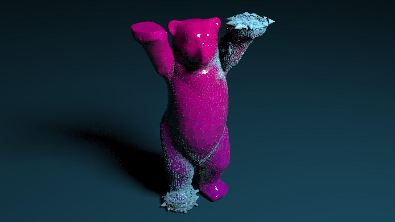
Below the electric potential on the buddy bear where we have placed a positive charge on its left upper paw and a negative charge under its right lower paw.
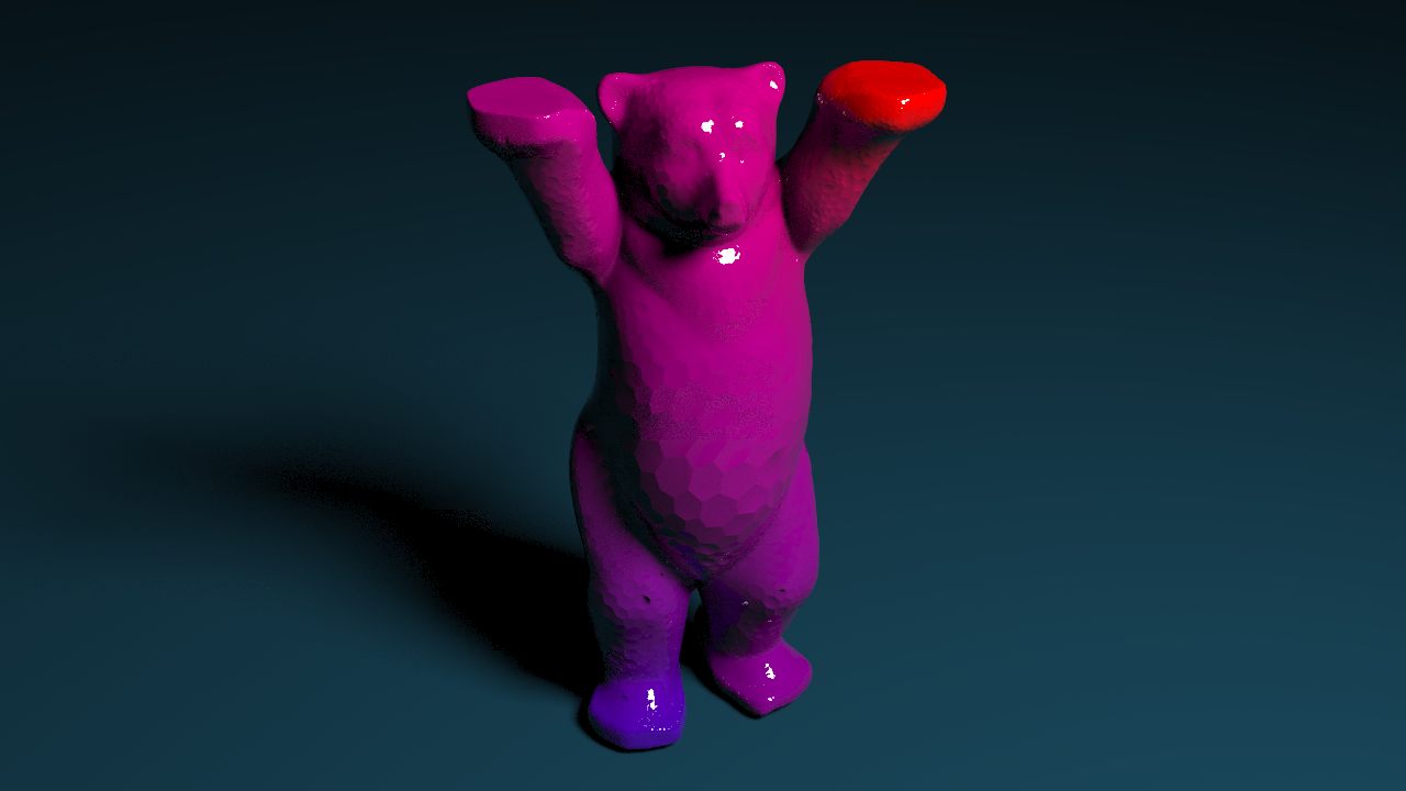
Actually the bear on the picture does not consist of triangles – we used a divide node to visualize the dual cells the piecewise constant functions live on.
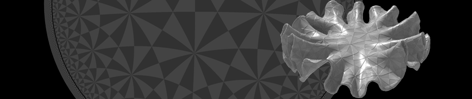
The graph of the function \(u\) (which is stored as a point attribute @u) can then be visualized by a polyextrude node. Therefore one selects Individual Elements in the Divide Into field and specifies the attribute u in the Z scale field.
The dual surface also provides a way to visualize the electric field: Once one has computed the gradient (on the primitives of the triangle mesh) the divide node turns it into an attribute at the points of the dual surface (corresponding to the actual triangles). This can then be used to set up attributes @pscale (length of gradient) and @orient (quaternion that rotates say \((1,0,0)\) to the direction of the gradient) and use them in a copy node to place arrows. Reading out the gradient at the vertices of the dual mesh needs a bit care:
vector g  = v@grad;
p@orient = dihedral(set(1,0,0),g);
@pscale = length(g);
Here how the end of the network might look like:
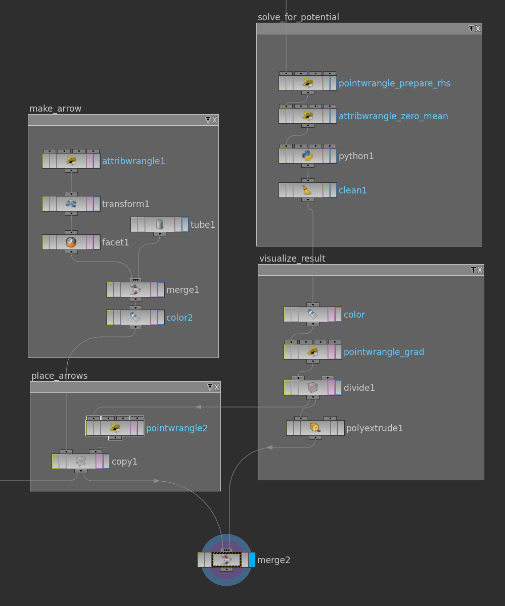
And here the resulting image:
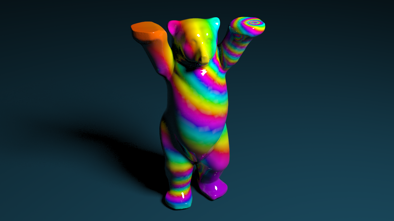
Since the potential varies quite smoothly the coloring from blue (minimum) to red (maximum) does not reveal much of the function. Another way to visualize \(u\) is by a periodic texture. This we can do using the method hsvtorgb, where we can stick in a scaled version of u in the first slot (hue).
Homework (due 11 June). Build a network that allows to specify the charge on a given geometry and computes the corresponding electric field and potential.