We are back at minimal surfaces in \(\mathbb S^3\). This time the goal is to visualize minimal surfaces in \(\mathbb S^3\) first described by Lawson, which are constructed by reflections and rotations of a fundamental piece which is a minimal surface spanned in a spherical quadrilateral, i.e. the solution of a spherical Plateau problem. So let us look at the Plateau problem in \(\mathbb S^n\).
Let \(M\) be a Riemannian surface with metric \(g\) and consider the \(n\)-sphere \(\mathbb S^n\) as subset of \(\mathbb R^{n+1}\). The Dirichlet energy of a map \(f\colon M \to \mathbb S^n\) is then given by the usual formula:\[E_D(f) = \tfrac{1}{2} \int_M |df|^2 = -\tfrac{1}{2} \int_M \langle f,\Delta^{\!g} f\rangle\,,\]where \(\Delta^{\!g}\) denotes the Laplacian operator defined for maps from \(M\) into \(\mathbb R^{n+1}\).
Though, if we restrict attention to maps into the \(n\)-sphere, the condition when a map is a critical point (harmonic) has changed: For a variation \(f_t\colon M \to \mathbb S^n\) of \(f\) with variational vector field \(Y_p =\tfrac{d}{dt}|_{t=0}f_t(p)\), we have\[\tfrac{d}{dt}|_{t=0}E_D(f_t) = -\int_M \langle Y,\Delta^{\!g} f\rangle\,.\]But, since \(|f_t|^2 = 1\), we have \(Y_p\perp f(p)\) for all \(p\) . Thus we conclude that a map \(f\colon M\to \mathbb S^n\) is harmonic, if and only if \(\Delta^{\!g} f = \rho f\) for some function \(\rho\colon M\to \mathbb R\).
For discrete functions into \(\mathbb S^n\) we adapt that to be the definition of harmonicity: Let \(M\) be a discrete Riemannian surface with metric \(\ell\) and let \(\Delta^{\!\ell}\) denote the corresponding cotan-Laplace operator, then a discrete map \(f\colon M \to \mathbb S^n\) is called harmonic, if\[\Delta^{\!\ell} f = \rho f\, \textit{ for some discrete function }\rho\colon M \to \mathbb R\,.\]
By the considerations above one easily finds that this definition actually amounts to defining the Dirichlet energy of a discrete function into the \(n\)-sphere to be the Dirichlet energy of the corresponding piecewise-linear function into \(\mathbb R^{n+1}\)—with only vertices mapped into the sphere. One finds then that a discrete map is harmonic if it is critical among these maps.
Note that the Dirichlet problem—given a map \(\gamma\colon \partial M \to \mathbb S^n\), find a harmonic map \(f\colon M \to \mathbb S^n\) such that \(f|_{\partial M} = \gamma\)—has become a non-linear problem. A simple idea to solve this problem is to average (with weights) and normalize alternatingly:
Let \(M\) be a discrete surface with edge length \(\ell\) and let \(\omega\) denote the corresponding cotangent weights. Let \(E\) denote the set of unoriented edges. Then, given a discrete map \(f^0\colon M \to \mathbb S^n\) such that \(f^0|_{\partial M} = \gamma\), we recursively define for interior vertices \(i\)\[f^{t+1}_j := \frac{\tilde f^{t+1}_j }{|\tilde f^{t+1}_j|}, \, \textit{ where }\,\tilde f^{t+1}_i := \sum_{\{i,j\}\in E} \omega_{ij} f^t_j\,,\]while boundary positions are unchanged, \(f^{t+1}_i = f^{t}_i= \gamma_i\) for all \(i\in \partial M\).
If \(f^\infty\colon M \to \mathbb S^n\) is the limit of this process, then it satisfies for each interior vertex \(i\)\begin{align*}f^\infty_i = \frac{\sum_{\{i,j\}\in E} \omega_{ij} f^\infty_j}{|\sum_{\{i,j\}\in E} \omega_{ij} f^\infty_j|} & \Leftrightarrow|\sum_{\{i,j\}\in E} \omega_{ij} f^\infty_j|\,f^\infty_i = \sum_{\{i,j\}\in E} \omega_{ij} f^\infty_j \\ & \Leftrightarrow (|\sum_{\{i,j\}\in E} \omega_{ij} f^\infty_j|-\sum_{\{i,j\}\in E} \omega_{ij})\,f^\infty_i = \sum_{\{i,j\}\in E} \omega_{ij} (f^\infty_j -f^\infty_i)\,,\end{align*}while it \(f^\infty|_{\partial M} = \gamma\). Thus \(f^\infty\) solves the Dirichlet problem.
Similarly to the Dirichlet energy we can define the area of a discrete map \(f\colon M \to \mathbb S^n\) to be the area of its piecewise-linear interpolation in \(\mathbb R^{n+1}\). With this definition we find that a discrete immersion \(f\colon M \to \mathbb S^n\) is minimal, if\[\Delta^{\!f} f = \rho f \, \textit{ for some discrete function }\,\rho \colon M \to \mathbb R\,.\]where \(\Delta^{\!f}\) denotes the cotan-Laplace operator with respect to the edge lengths \(\ell_{ij} = |f_j- f_i|\) induced by \(f\).
The algorithm to solve the Dirichlet problem can be easily modified to solve the Plateau problem—just update edge lengths in each step.
To produce Lawson’s minimal surfaces we need to solve then the Plateau problem for geodesic quadrilaterals \(\square_{k,m}=P_1Q_qP_2Q_2\) in \(\mathbb S^3\), where\[P_1,P_2 \in C_1 = \{(z,w)\in \mathbb S^3 \subset \mathbb C^2 \cong \mathbb R^4 \mid |z| = 1\},\quad \mathrm{dist}(P_1,P_2) = \frac{\pi}{k+1}\]and\[Q_1,Q_2 \in C_2 = \{(z,w)\in \mathbb S^3 \subset \mathbb C^2 \cong \mathbb R^4 \mid |w| = 1\},\quad \mathrm{dist}(Q_1,Q_2) = \frac{\pi}{m+1}\,.\]Let us restrict attention only to the case \(m=1\). In this case \(k\) is just the number of handles—the genus of the surface.
Under the stereographic projection the quadrilateral \(\square_{k,1}\) look as follows
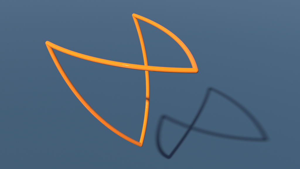
For the figure used the stereographic projection from northpole \(e_4\in \mathbb R^4\) where the square \(\square_{k,1}\) (here \(k=2\)) was sampled by the discrete curve \(\gamma\colon \mathbb Z/4n\mathbb Z \to \mathbb C^2\) with \(4n\) vertices given by\[\gamma_j = \cases{\Bigl(\cos(\tfrac{\pi j}{2n})\mathbf 1,\sin(\tfrac{\pi j}{2n})\mathbf e^{-\tfrac{\pi\mathbf i}{4}}\Bigr) & for \(0\leq j\,\%\,4n<n\) \\\Bigl(\cos(\tfrac{\pi j}{2n})\mathbf e^{\pi\mathbf i – \tfrac{\pi\mathbf i}{k+1}},\sin(\tfrac{\pi j}{2n})\mathbf e^{-\tfrac{\pi\mathbf i}{4}}\Bigr) & for \(n\leq j\,\%\,4n < 2n\) \\\Bigl(\cos(\tfrac{\pi j}{2n})\mathbf e^{\pi\mathbf i – \tfrac{\pi\mathbf i}{k+1}},\sin(\tfrac{\pi j}{2n})\mathbf e^{\tfrac{\pi\mathbf i}{4}}\Bigr) & for \(2n\leq j\,\%\,4n<3n\) \\\Bigl(\cos(\tfrac{\pi j}{2n})\mathbf 1,\sin(\tfrac{\pi j}{2n})\mathbf e^{\tfrac{\pi\mathbf i}{4}}\Bigr) & for \(3n\leq j\,\%\,4n<4n\)}\,.\]In Houdini we can easily implement this formula starting with a circle node with \(4n\) vertices and store the points of \(\square_{k,1}\) as vector4 point attribute p@f using a point wrangle node.
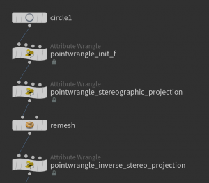
Now given the boundary polygon we want to have a surface \(f\) to start with. Usually we can get such surface using a remesh node. Unfortunately this node only works on point positions in \(\mathbb R^3\). Though it also interpolates the values of p@f which then can be normalized, it turns out to be better to remesh instead the stereographic projection which then can be mapped back to the \(3\)-sphere using the inverse stereographic projection. Here how the network might look at this point:
Furthermore we again need to identify interior points. This e.g. can be done by a sequence of group nodes:
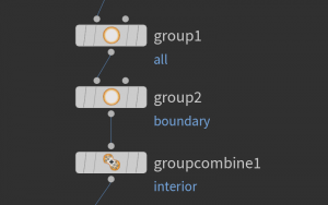
Here the first group node just collects all the points by the base group option. The second only selects boundary vertices, which then are subtracted from the first group using a group combine node.
Now we are ready to iterate. This can be done by a loop node as we already used or—if one is interested in the progress of the iteration using a solver node

which performs one step per frame when then play button at the lower left corner is hit. The network inside look as follows:

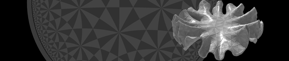
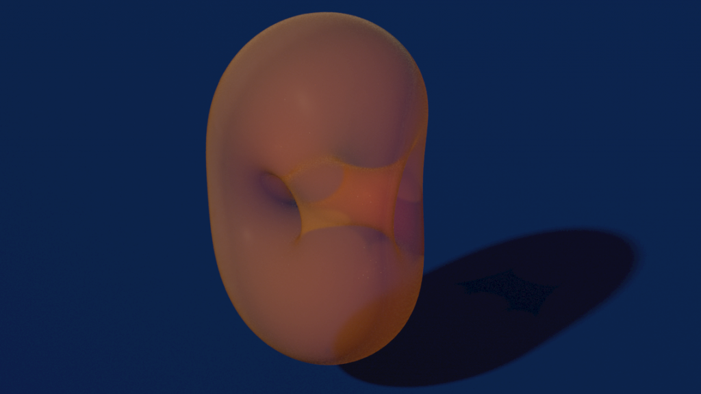
Here the cotangent weight of the current immersion are computed using vertex wrangle nodes. After that we use point wrangle node on the interior point group to perform the iteration on the vector4 attribute p@f. Here a sequence of frames how the results may look like:
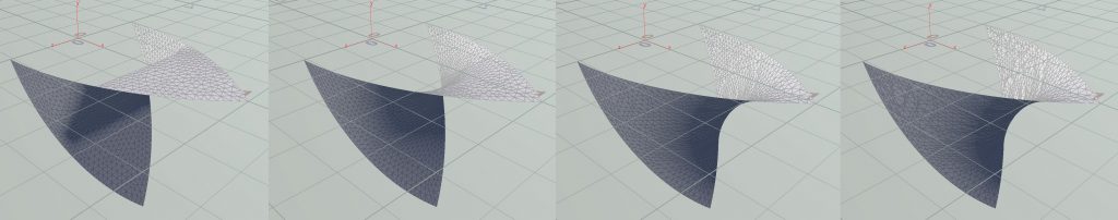
The first picture shows the first frame while the last shows the 2000th.
After we solved the Plateau problem we can rotate and reflect the quadrilateral to form a larger piece. This is done here in a subnetwork which at the end spits out the stereographic projection
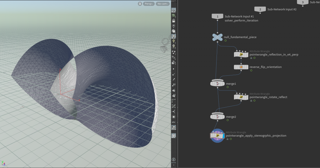
Here the point wrangle node reflect_in_e4_perp multiplies the 4th component of p@f by \(-1\). The second also contains just one line as well
p@f = set(p@f[0],-p@f[1],-p@f[3],p@f[2]);
The resulting patch can then be copied and rotated \((k+1)\)-times around the \(z\)-axis to form the Lawson surface. Using a fuse node we can even turn the patches into a single closed surface which then can be remeshed if needed:
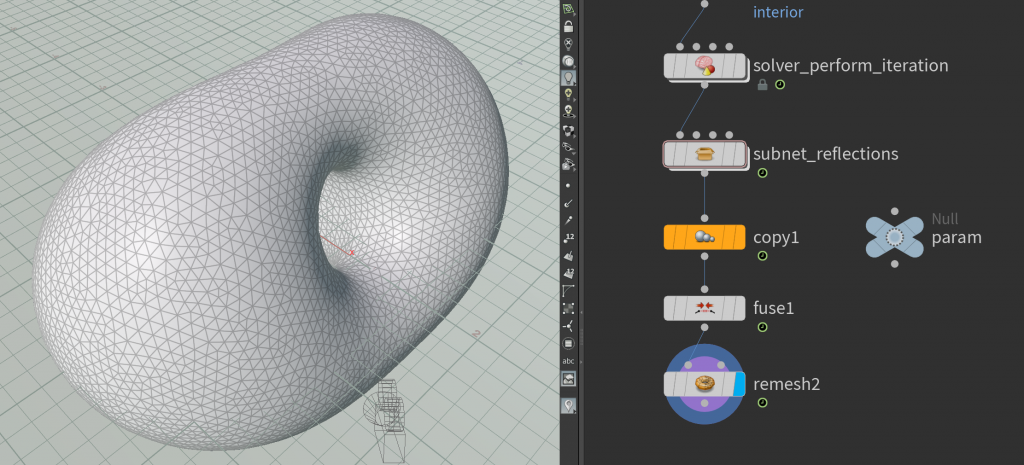
Here you also see a null node to globally store the parameters \(k\) and \(n\).
In particular we are now able to produce closed minimal surfaces in the \(3\)-sphere of arbitrary genus. Here a Lawson surface of genus \(7\):
Homework (due 18 June). Build a network that computes for a given \(k>0\) the corresponding Lawson surface.