Let \(M\) be a Riemannian surface and let \(\Delta\colon C^\infty M \to C^\infty M\) denote the corresponding Laplace operator. The second order linear partial differential equation \[\ddot{u} = \Delta u\]is called the wave equation and—as the name suggests—describes the motion of mechanical or light waves. The goal of this tutorial is to visualize waves on surfaces.
For a discrete surface \(M\) with given edge lengths we know how to build up the Laplace operator. To solve the wave equation we will use the so called Verlet integration scheme. It has very nice properties and is very simple.
To obtain the Verlet scheme one just approximates the second derivative of the function \(u\) as follows: For a given fixed time step \(0<\varepsilon \in\mathbb R\),\[\ddot u (t) \approx \frac{1}{\varepsilon}\Bigl(\frac{u(t+\varepsilon) – u(t)}{\varepsilon} -\frac{u(t) – u(t-\varepsilon)}{\varepsilon}\Bigr) = \frac{u(t+\varepsilon) – 2u(t) +u(t-\varepsilon)}{\varepsilon^2}\,.\]Thus we can compute \(u(t+\varepsilon)\) from \(u(t-\varepsilon)\) and \(u(t)\):\[u(t+\varepsilon) = \varepsilon^2\Delta u(t) + 2u(t) – u(t-\varepsilon)\,.\]So, given \(u(t_0),u(t_1)\), \(t_1 = t_0+\varepsilon\), this recursively defines the whole discrete time evolution \(u(t_i)\), \(t_i = t_0 + i\varepsilon\).
Note that in the discrete setting the space of piecewise linear functions is finite dimensional and, if \(V\) is the set of vertices, can be identified with \(\mathbb R^V \cong\mathbb R^n\), \(n = |V|\). The wave equation has become an ordinary differential equation which has a unique solution for given initial data \(u(t_0),\dot u (t_0)\). For the time discrete flow \(\dot u (t_0)\) is replaced by \(u(t_1)\). Though the solution space has the same dimension as in the continuous setting.
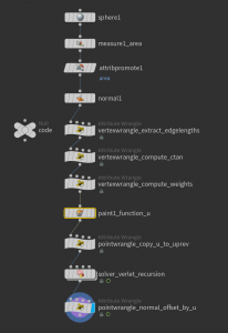
We can easily build up a network to solve the wave equation on closed surfaces. Let us start here with a sphere on which we paint a function stored as a point attribute u, which plays the role of \(u(t_1)\). Then we copy u to a second attribute uprev playing the role of \(u(t_0)\)—this basically amounts to setting the initial velocity to zero. Then we implement the Verlet step by a solver node (containing a single pointwrangle node) and display the result by either colors of some normal offset. That is again easily done by one line in a pointwrangle node (v@P += f@u*v@N). Here the complete network:
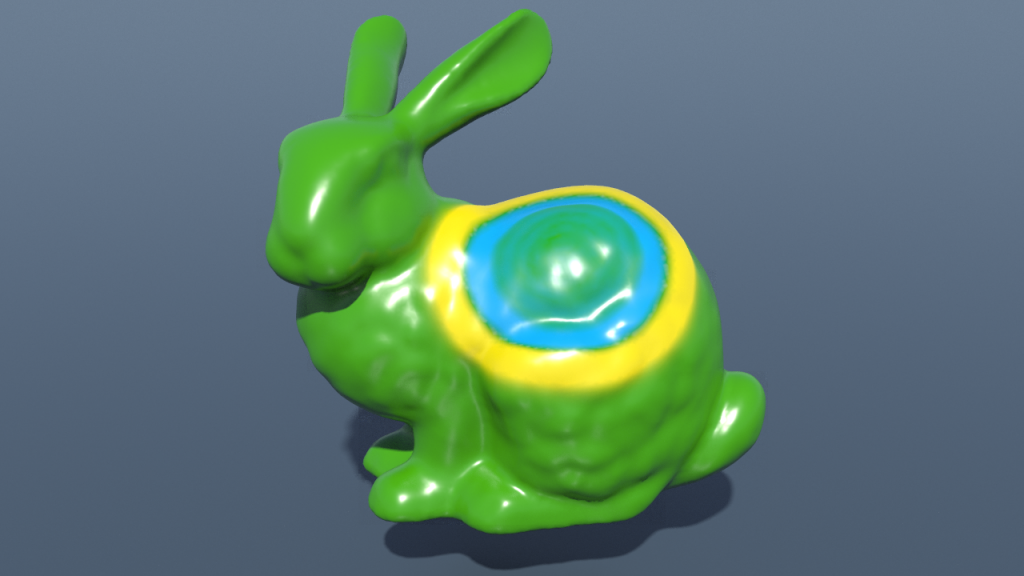
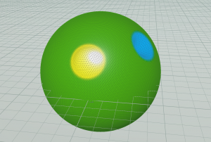
Below you find an example how the initial \(u\) might look like using both—normal offset and color coding.
A movie of how the evolution looks like you can find here. Note that the bumps really almost reappear.
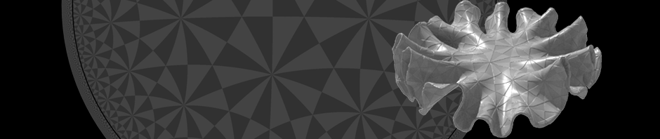
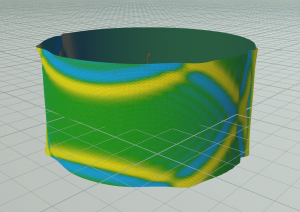
For surfaces with boundary we need to specify what happens at the boundary. One way to deal with boundary is to glue a reflected copy of the surface along the boundary—so one gets a closed surface without boundary but with a reflectional symmetry—and restrict the attention only to functions invariant under the reflection. Practically this means to do nothing special: For boundary edges there is only one cotangent so we have double it. Each edge which is not a boundary edge but ends at a boundary vertex appears with the same weights on the copy. So these appear twice in the sum as well. But also the area is doubled. So if we divide by area nothing changes. As a result the waves are reflected at the boundary, as shown in the picture below.
Here the corresponding video.
Homework (due 25 June). Build a network that simulates waves on surfaces.