In previous tutorials we compute immersed minimal surfaces. These immersions were the critical points of Dirichlet energy. You have seen in the lecture that, if we additionally include a volume constraint, then the critical points have no longer mean curvature \(H=0\) but it is constant—we obtain so called constant mean curvature (CMC) surfaces.
Let \(M\) be a surface. On the space of immersion \(f\colon M\to \mathbb R^3\) we consider for fixed \(p \in \mathbb R\) the energy\[\mathbf E_p(f) = E_D (f) + p V(f)\,,\]where\[E_D(f)= \tfrac{1}{2}\int_M |df|^2,\quad V(f) = \tfrac{1}{6}\int_M \langle f, df\times df\rangle\,,\]i.e. \(E_D(f)\) is the Dirichlet energy of \(f\) and \(V(f)\) the volume ‘enclosed’ by \(f\).
If we look at the critical points of \(\mathbf E_\lambda\) we find that these are CMC immersions: As seen in the lecture, we have\[ \dot{E}_D = \int_M \langle -\Delta^g f,\dot f\rangle,\quad \dot V = \int_M \langle N,\dot f\rangle\,.\]Moreover, \(\Delta^g f = -2HN\). Thus\[\mathrm{grad}_f\,\mathbf E_p = -\Delta^g f + p N = (2H +p) N\,.\]Thus a critical point \(f\) satisfies \(H = -p/2\).
So if we minimize for a given fixed \(p\) the energy \(\mathbf E_\lambda\) we obtain a CMC surface. One way to minimize is gradient descent. As explained in this fabulous article another and actually better method to minimize is the so-called momentum method—it guarantees faster convergence. So we are left to solves the following second order equation\[\ddot f + \rho\dot f = \Delta^g f + p N\,\]for some damping constant \(\rho>0\).
The equation above also has a nice Newtonian interpretation: By Newtons second law the above equation describes a surface on which act two forces—surface tension \(\Delta^g f\) and pressure \(pN\).
For the second derivative we use the same ansatz as last time and the first derivative is approximated by a difference quotient: For given stepsize \(\varepsilon >0\),\[\frac{f(t+\varepsilon) – 2f(t) +f(t-\varepsilon)}{\varepsilon^2} + \rho\frac{f(t) –f(t-\varepsilon)}{\varepsilon} = \Delta^{g(t)} f(t) + \lambda N(t)\,.\]Rearranging terms yields\[f(t+\varepsilon) =\varepsilon^2 \bigl(\Delta^{g(t)} f(t) +\lambda N(t)\bigr) +2f(t) – f(t-\varepsilon) – \rho\varepsilon (f(t)-f(t-\varepsilon))\,.\]Note that here—in contrast to last time—the Laplace operator depends on \(t\) as well.
One might be tempted to approximate the first derivative by a more symmetric expression like the average of difference quotients, but this is doomed. As Albert explained to me, that’s well known—e.g. if one discretizes the left hand side of the diffusion equation \(\dot u = \Delta u\) by the average of difference quotients the system becomes unconditionally unstable, i.e. no matter what \(\varepsilon\) one chooses the equation is unstable.
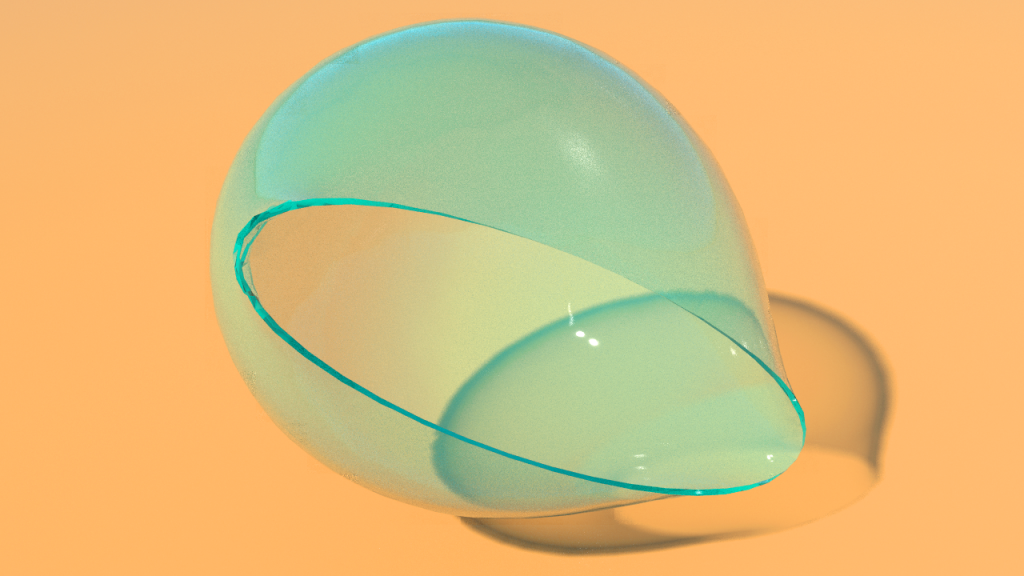
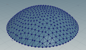
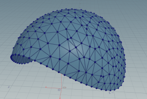
Let \(M\) be a surface with boundary. Minimization of \(E_p\) for a suitably chosen pressure \(p\) among all immersions which have the same boundary curve \(\gamma\) seems to work quite nicely. E.g. a flat disk is flowing to a spherical cap as show in the picture below.
As a short video shows, the method converges quickly.
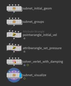
Here the corresponding network—it just prepares the initial conditions and implements the flow using a solver node.
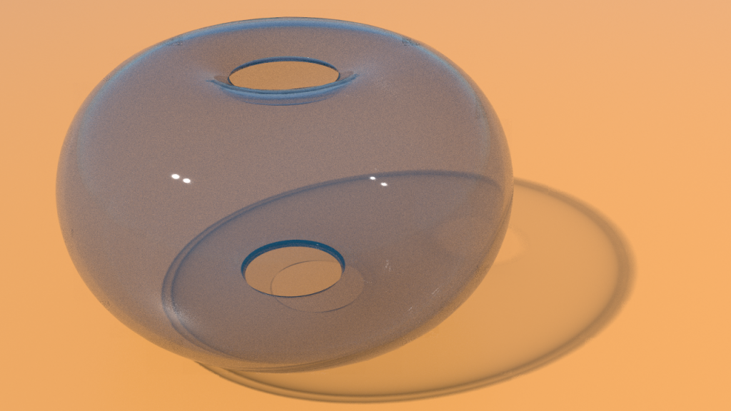
More interestingly, this also works for more generic boundary curves producing CMC surface which are no longer a part of a sphere.
In principle triangles can degenerate during the flow. To prevent them from becoming too bad we just used a polydoctor node (inside the solver) to repair the mesh if it becomes necessary. Not all situations can be fixed this way but it often help a lot.
For small pressure \(p\) the surface tension and pressure can balance and we end up with a CMC surface. For large \(p\) this is no longer true and the surface just blows up—we just pump more and more air ‘into’ the surface.
From physics we know that pressure is not constant—the ideal gas law says that, up to physical constants,\[pV = T,\]where \(T\) denotes temperature. It is worth to look at the dynamics one gets if we fix \(T\) and include the dependence of \(p\) on \(V\) in the force. Here a movie of an ellipsoid with some downward pointing impulse moving according to the equations of motion.
Let us come back to the problem of computing CMC surfaces. Therefore let us now impose a hard volume constraint, i.e. we minimize Dirichlet energy over all immersions which satisfy\[C(f) := V(f) – V_0 = 0\] for a given fixed \(V_0\in \mathbb R\). Such constraint optimization problems can be tackled by the so-called augmented Lagrangian method (ALM). Here \(\lambda\) is modified during the minimization: For a given initial \(\lambda\in \mathbb R\) iterate
- for fixed \(\lambda\), minimize the unconstraint problem\[\mathbf E_{aug}(f) = E_D(f) + \tfrac{1}{2}C(f)^2 +\lambda C(f)\,,\]
- use the minimizer \(f_0\) to update \(\lambda\) \[\lambda \gets \lambda + C(f_0)\,.\]
If we don’t minimize to the very end in the first step, but instead change it to a finite amount of gradient descent, and interpret the update of \(\lambda\) as a forward Euler step we obtain the continuous system:\begin{align*}\dot f & = \Delta^g f – (\lambda+C(f)) N\,,\\ \dot \lambda &=C(f)\,,\end{align*}where \(N\) denotes the Gauss map of \(f\)—which is the gradient of the volume functional \(V\).
Now let us look at a stationary point \(f\) of this continuous system: \(\dot \lambda = 0\) implies that \(V(f) = V_0\). From \(\dot f = 0\) then follows \(0 = \Delta^g f – \lambda N\). Thus we have\[2H\, N = -\Delta^g f = -\lambda N\,.\]So a stationary point \(f\) is just a CMC surface with mean curvature \(H=-\lambda/2\).
Let us again change the first line of the system above to second order with damping. The final system then becomes\begin{align*}\ddot f + \rho\dot f & = \Delta^g f – (\lambda + C(f)) N\,,\\ \dot \lambda &=C(f)\,,\end{align*}for some damping constant \(\rho>0\). Again the stationary points are CMC.
So, for a given stepsize \(\varepsilon >0\), we finally do the following updates: \[f(t+\varepsilon) = \varepsilon^2 \bigl(\Delta^{g(t)} f(t) – (\lambda(t)+C(f(t))) N(t)\bigr) +2f(t) – f(t-\varepsilon) – \rho\varepsilon(f(t)-f(t-\varepsilon))\,,\]followed by\[\lambda(t+\varepsilon) = \lambda(t) + \varepsilon C(f(t+\varepsilon))\,.\]
This all translates nicely to the discrete case–the Laplace operator is given by cotangent weights and the gradient the volume is the vertex normal field \(N\) which at a vertex \(i\) is given by the area vector of the boundary of the vertex star (the \(1\)-link), i.e. if \(j_1,\ldots,j_n=j_0\) denote the neighboring vertices of \(i\) ordered counter-clockwise, then\[N_i = A_i/|A_i|, \textit{ where } A_i = \tfrac{1}{2}\sum_{k=0}^{n-1} (f_{j_k}-f_i)\times (f_{j_{k+1}} – f_i)\,.\]
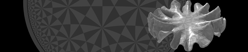
Here a movie of the dynamics of a flat ellipsoid blowing up to the CMC surface in the teaser image. The method is not restricted to disks. Below you find an image of a CMC cylinder.
Homework (due 2 July). Build a network which flows a given surface to a CMC surface of prescribed volume.