Conformal Maps III: Stereographic Projection

Stereographic projection

\[\sigma: \mathbb{R}^n \to S^n \setminus \{\mathbf{n}\}\]

where

\[\mathbf{n}=(0,\ldots,0,1)\in\mathbb{R}^{n+1}\]

is the northpole of $S^n$ is a special case of an inversion: Let us consider the hypersphere $S\subset\mathbb{R}^{n+1}$ with center $\mathbf{n}$ and radius $r=\sqrt{2}$ and look at the image of

\[\mathbb{R}^n =\left\{\mathbf{x}\in\mathbb{R}^{n+1}\,{\large |}\, x_{n+1}=0\right\}\]

under the inversion $g$ in $S$. The points in the image $g(\mathbb{R}^n)$ satisfy

\begin{align*}0&=\left\langle \mathbf{n},\mathbf{n}+2\,\frac{\!\!\!\mathbf{x}-\mathbf{n}}{|\mathbf{x}-\mathbf{n}|^2}\right\rangle\\\\&=\frac{|\mathbf{x}|^2-1}{|\mathbf{x}|^2+1}\end{align*}

And therefore lie on the unit sphere $S^n$. With the notation $\sigma:=\left.g\right|_{\mathbb{R}^n}$ we obtain

\[\sigma(\mathbf{x})=\frac{2\mathbf{x}+(|\mathbf{x}|^2-1)\mathbf{n}}{|\mathbf{x}|^2+1}.\]

Let us compute also $\sigma^{-1}=\left.g\right|_{S^n \setminus \{\mathbf{n}\}}$. For $\mathbf{x} \in S^n \setminus \{\mathbf{n}\}$ we have

\[\sigma^{-1}(\mathbf{x})=\frac{\mathbf{x}-\langle \mathbf{n},\mathbf{x}\rangle \mathbf{n}}{1-\langle \mathbf{n},\mathbf{x}\rangle}.\]

Note that we have

\[\sigma(\mathbf{x})=\lambda \mathbf{x}+\mu \mathbf{n}\]

with $\lambda+\mu=1$. This means that $\mathbf{n}$, $\mathbf{x}$ and $\sigma(\mathbf{x})$ always lie on a straight line. This accounts for the fact that $\sigma$ is called a projection with the north pole as its center. There is a beautiful video by Henry Segerman that illustrates stereographic projection by placing an LED at the north pole of a 3D-printed sphere and watching the shadow on a horizontal plane.

stereographic

Here the plane on which $\sigma$ is defined touches the sphere, whereas in  our case it cuts the sphere in the equator. This is of course irrelevant. Here is another video with more patterns.

Posted in Lecture | Leave a comment

Conformal Maps II: Inversions

Let $M\subset \mathbb{R}^n$ be a domain. A smooth map $f:M \to \mathbb{R}^n$ is called conformal if there is a smooth function $\phi:M\to \mathbb{R}$ and a smooth map $A$ from $M$ into the group $O(n)$ of orthogonal $n\times n$-matrices such that the derivative $f’$ of $f$ satisfies

\[f’=e^\phi A.\]

In the two dimensional case this definition agrees with the one given in an earlier post. It means that when restricting attention to very small regions (i.e. looking through a microscope) $f$ looks like a similarity transformation. The similarity transformations themselves, defined as affine maps of the form

\begin{align*}f:\mathbb{R}^n &\to \mathbb{R}^n \\\\ f(\mathbf{x}) &=e^\phi A \mathbf{x}+\mathbf{b}\end{align*}

with $\phi\in\mathbb{R}$, $A\in O(n)$, $\mathbf{b}\in\mathbb{R}^n$ are standard examples of conformal maps.

The theory of holomorphic functions shows that for $n=2$ there is an abundance of conformal maps $f$ from domains in $M\subset \mathbb{R}^n$ into $\mathbb{R}^n$. In contrast, a famous theorem proved by Liouville in 1850 says that for $n \geq 3$ all such maps $f$ are of the form

\[f= s_1\circ g \circ s_2\]

where $s_1$ and $s_2$ are similarity transformations and

\begin{align*}g:\mathbb{R}^n\setminus\{\mathbf{o}\} &\to \mathbb{R}^n\setminus\{\mathbf{o}\} \\\\ g(\mathbf{x}) &=\frac{\!\!\!\mathbf{x}}{|\mathbf{x}|^2}\end{align*}

is the so-called inversion in the unit sphere $S^{n-1}$. Inversion interchanges the exterior of $S^{n-1}$ with its interior (from which the origin has been removed). All points of $S^{n-1}$ are fixpoints of $g$. For this reason $g$ is also called the reflection in the unit sphere.

Let us prove that $g$ is conformal. For all $\mathbf{x}\in\mathbb{R}^n\setminus\{\mathbf{o}\}$ and $\mathbf{y}\in \mathbb{R}^n$ we have

\begin{align*}g'(\mathbf{x})\,\mathbf{y}&=\frac{\!\!\!\mathbf{y}}{|\mathbf{x}|^2}-\frac{2\langle \mathbf{x},\mathbf{y}\rangle}{|\mathbf{x}|^4}\\\\ &=\frac{\!\!\!1}{|\mathbf{x}|^2}\left(\mathbf{y}-2\left\langle \frac{\mathbf{x}}{|\mathbf{x}|},\mathbf{y}\right\rangle\frac{\mathbf{x}}{|\mathbf{x}|}\right).\end{align*}

Now the map

\[\mathbf{y} \mapsto A\mathbf{y}:=\mathbf{y}-2\left\langle \frac{\mathbf{x}}{|\mathbf{x}|},\mathbf{y}\right\rangle\frac{\mathbf{x}}{|\mathbf{x}|}\]

is reflection in the unit vector $\frac{\mathbf{x}}{|\mathbf{x}|}$ and therefore orthogonal. Thus $g$ is conformal. Here is what happens if we apply $g$ to a small cube inside the unit sphere:

 inversion-3

Apparently, all cube faces are mapped to pieces of round spheres. Let us prove this in general: If we have a hyperplane

\[E = \{\mathbf{x}\in \mathbb{R}^n \,|\,\langle \mathbf{x},\mathbf{n}\rangle = d\}\]

with unit normal $\mathbf{n}$ and distance $d\neq 0$ to the origin, then all points $\mathbf{x}\in g(E)$ satisfy

\begin{align*}0&=\left\langle\frac{\!\!\!\mathbf{x}}{|\mathbf{x}|^2},\mathbf{n}\right\rangle -d\\\\&=-\frac{\!\!\!d}{|\mathbf{x}|^2}\left(\left\langle \mathbf{x} -\frac{\mathbf{n}}{2 d},\mathbf{x}-\frac{\mathbf{n}}{2 d}\right\rangle -\frac{1}{4 d^2}\right).\end{align*}

So they lie on the sphere with center $\frac{n}{2d}$ and radius $\frac{2d}$. A similar computation shows that any piece of a sphere or plane that does not contain the origin is mapped onto a piece of another sphere or plane. Since planes can be regarded as limiting cases of spheres, a concise though slightly sloppy way to express this fact is by saying that “$g$ transforms spheres into spheres”.

The inversion in a sphere with center $\mathbf{m}$ and radius $r$ is defined as

\[\mathbf{y}\mapsto \mathbf{m}+\frac{\!\!\!\mathbf{y}-\mathbf{m}}{\left|\mathbf{y}-\mathbf{m}\right|^2}.\]

Posted in Lecture | Leave a comment

Conformal Maps I: Holomorphic Functions

If $M\subset\mathbb{R}^2$ is a plane domain and the image of parametrized surface $f:M\to \mathbb{R}^3$ is contained in

\[\mathbb{R}^2=\{(x,y,z)\in \mathbb{R}^3\,\,|\,\, z=0\}\]

then the defining equations of a conformal map

\begin{align*}\left|f_u\right|&=\left|f_v\right| \\\\ \langle f_u,f_v\rangle &=0\end{align*}

imply that $\left|f_v\right|$ arises from $\left|f_v\right|$ by a $90^\circ$-rotation, either counter-clockwise,

\[f_v=J\,f_u\]

or clockwise:

\[f_v=-J\,f_u.\]

Here

\[J = \left(\begin{array}{cc}0 & -1 \\ 1 & 0\end{array}\right)\]

is the matrix corresponding to the $90^\circ$-rotation in the positive sense. Let us stick to the first possibility $\left|f_v\right|=J\left|f_u\right|$ which corresponds to the case where the map $f$ preserves orientation. If you spell out what this property means for the two component functions of $f$, you will find this relation to be equivalent to the Cauchy-Riemann equations. So, if we identify $\mathbb{R}^2$ with the set $\mathbb{C}$ of complex numbers, orientation-preserving conformal maps from domains in $\mathbb{R}^2$ into $\mathbb{R}^2$ are holomorphic maps. Note that the above matrix $J$ has the same effect on vectors in $\mathbb{R}^2=\mathbb{C}$ as multiplication by $i$.

The above observation supplies us with a rich source for conformal parametrizations. At least away from the zeros of their derivative, all holomorphic maps are conformal. For example, all complex polynomials are conformal. Below we show the map

\begin{align}f: M &\to \mathbb{C} \\ f(z) &= \frac{z^4}{4}-z\end{align}

where $M$ is a certain annulus (shown in white). To help orientation in $\mathbb{C}$, we also displayed the unit circle. Not that the roughly square-shaped quadrilaterals of the annulus approximately retain their shape, basically they are only scaled.

holomorphic

Posted in Lecture | Leave a comment

Conformal Parametrizations of Surfaces

In the context of surfaces the strict analog of arclength parametrized curves is an isometric immersion

\[f: M\to \mathbb{R}^3\]

of a standard surface into $\mathbb{R}^3$. Here “isometric” means that lengths of curves and intersection angles of curves on the surface remain the same as they were on the standard surface $M$. As an example, here is an isometric immersion of an annulus in $\mathbb{R}^2$:

isometric-2

Here we used in a Point Wrangle node the following VEX code that wraps the $z,x$-plane isometrically around a cone:

#include "Math.h"

float alpha = PI/180 * ch("alpha");
float ca = cos(alpha);
float sa = sin(alpha);
float z = @P.z;
float x = @P.x;
float r = sqrt(z*z + x*x);
float phi = atan2(z,x)/ca;
@P.z = ca * r * cos(phi);
@P.x = ca * r * sin(phi);
@P.y = sa * r;

If the parameter domain is a subset $M\subset \mathbb{R}^2$, the standard coordinates of $\mathbb{R}^2$ are labeled $u,v$ and subscripts denote partial derivatives then $f$ is isometric if and only if

\begin{align*}\left|f_u\right|=\left|f_v\right|&=1 \\\\ \langle f_u,f_v\rangle &=0.\end{align*}

Very few surfaces admit such an isometric parametrizations. Also the possible isometric deformations of a given surface in $\mathbb{R}^3$ are quite limited and rigid. We therefore look at the larger class of conformal deformations, which preserve intersection angles of curves on the surface but not the length. So local features are enlarged or shrunk but not distorted.

conformal

A parametrization $f$ defined on a domain $M\subset \mathbb{R}^2$ is conformal if and only if the exists local scalings  $e^\phi$ defined by a function $\phi: M \to \mathbb{R}$ such that

\begin{align*}\left|f_u\right|=\left|f_v\right|&=e^\phi \\\\ \langle f_u,f_v\rangle &=0.\end{align*}

For many applications (including numerical computations) it is desirable that the triangles of a simplicial surface are as equilateral as possible. Similarly often the quadrilaterals of a quadrilateral mesh should preferably as square-shaped as possible. Conformal deformations have the pleasant feature that they do not deteriorate the quality of the mesh (when measured in this sense).

Posted in Lecture | Leave a comment

Structure derived from Halfedges

The halfedge description $M=(E,s,\rho)$ of an oriented surface contains all the information. It is nevertheless convenient to introduce some more derived stucture. For an edge $e\in E$ we define

$\textrm{left}(e)=$ the face (cycle of $s$) containing $e$

$\textrm{right}(e)=$ the face (cycle of $s$) containing $\rho(e)$

$\textrm{start}(e)=$ the vertex (cycle of $s\circ\rho$) containing $e$

$\textrm{end}(e)=$ the vertex (cycle of $s\circ\rho$) containing $\rho(e)$

$\textrm{unorient}(e)=$ the unoriented edge (cycle of $\rho$) containing $e$.

Denote by $F$ the set of all faces of $M$, by $V$ the set of all vertices and by $\tilde{E}$ the set of all unoriented edges.

If we look at the quintuple $(E,V,\rho,\textrm{start},\textrm{end})$ we see finite sets $E,V$, an involution $\rho: E \rightarrow E$ without fixed points and two maps $\textrm{start},\textrm{end}: E \rightarrow V$ such that

$\textrm{start} \circ \rho = \textrm{end}$

This is a one of the possible descriptions of a general finite graph. This graph is called the 1-skeleton or edge-graph of $M$. In a computer graphics context one might also call it the wireframe of $M$.

Posted in Lecture | Leave a comment

The two most Simple Discrete Surfaces

We claim that any pair of permutations $s,\rho$ of a finite set $E$ (with $\rho$ involutive and without fixpoints) defines a unique cell decomposition of some compact surface without boundary. No further conditions are needed. To illustrate this, we look at the simplest possible cases where $E=\{e,\tilde{e}\}$ has only two elements. Then necessarily $\rho(e) = \tilde{e}$ and $\rho(\tilde{e})=e$. For $s$ we have two possibilities:

1) $s=id_E$. Then we have two faces, the first one $\varphi$ being bounded by the single edge $e$, the second one $\tilde{\varphi}$ bounded by $\tilde{e}$. We have $s\circ \rho = \rho$ and therefore only one vertex $v$. This is a cell-decomposition of the sphere as shown in the picture below.

2) $s=\rho$. Then we have only one face bounded by the the edge $e$ followed by the edge $\tilde{e}$. We have $s\circ \rho = id_E$ and therefore two vertices $v$ (with a single outgoing edge $e$) and $\tilde{v}$ (with a single outgoing edge $\tilde{e}$). This is also a cell-decomposition of the sphere.

Posted in Lecture | Leave a comment

Halfedge Description of Oriented Surfaces

Imagine a cell decomposition $M$ of an oriented compact surface without boundary. Denote by $E$ the set of all oriented edges of $M$. Then for each $e \in E$ there is a unique face $\varphi$ on the left of $e$. Denote by $s(e)$ the oriented edge following $e$ in the cycle of oriented edges in the boundary of $\varphi$. Then

$s: E \rightarrow E$

is a bijective map (a permutation of the elements of $E$). Denote by

$\rho: E \rightarrow E$

the map that assigns to $e$ the same edge with the opposite orientation. Then $\rho$ has no fixed points and satisfies

$\rho^2 = \textrm{id}_E$.

We claim that the whole cell-decomposition can be uniquely recontructed from the permution $s$ and the involution $\rho$ without fixed points: The set of faces $F$ can be recovered from $s,\rho$ as the set of cycles of $s$. A cycle of $s$ is a subset $\varphi \subset E$ which is invariant under $s$ (meaning $s(\varphi)  = \varphi$) that cannot be decomposed in any way into smaller invariant subsets. Similarly, the outgoing oriented edges from a vertex $v$ are cycles of the permutation

$s\circ \rho : E \rightarrow E$.

Finally, unoriented edges $\epsilon$ are represented as cycles of $\rho$.

Posted in Lecture | Leave a comment

Combinatorial Geometry: Cell Complexes

Roughly speaking, Combinatorial complexes play a similar role in the discrete world as differentiable manifolds in the smooth world. They are able to capture the “intrinsic” properties of a geometric object, i.e. those properties that are independent of any embedding into an ambient space.  Combinatorial complexes come in two flavors: cell complexes and simplicial complexes. In this post we deal with the former.

A one-dimensional combinatorial cell complex is the same thing as a finite multigraph. Such a multigraph $M$ is given by

  • a finite set $P$ of “points”.
  • a finite set $\tilde{E}$ of “oriented edges”.
  • maps $s,d: \tilde{E}\to P$ assigning to each oriented edge its “source point” $s(e)$ and its destination point $d(e)$.
  • a map $\rho: \tilde{E}\to \tilde{E}$ that implements “orientation reversal”: We demand that for all $e\in\tilde{e}$ we have $\rho(e)\neq e$ and $\rho\circ \rho(e)=e$. Moreover we assume

\begin{align}s\circ \rho &= d \\ d\circ \rho &= s.\end{align}

Note that what we call “points” usually would be called “vertices”. We use “points” in order to remain consistent with Houdini terminology. A two-element subset $\hat{e}\subset\tilde{E}$ of the form $\{e,\rho(e)\}$ is called an (unoriented) edge of $M$.

A typical multigraph looks like this:

Multi-pseudograph

You see that there can be several edges connecting the same pair of points and there can be oriented edges whose source and destination point coincide. There also could be isolated points that do not belong to any edge.

A two-dimensional combinatorial cell complex is a one-dimensional cell complex $G$ together with a set $F$ of faces, where to each face $\varphi$ there is assigned a corresponding “edge cycle” of $G$. What is an edge cycle?

An edge loop in a one-dimensional cell complex $G$ is a finite sequence $(e_1,\ldots,e_n)$ of oriented edges in $G$ such that for $1\leq j\leq n$ we have

\[d(e_j)=s(e_{j+1})\]

and $d(s_n)=s(e_1)$. An oriented edge cycle in $G$ is an equivalence class of edge loops where two edge loops are considered equivalent if they only differ by a cyclic permutation of the edges. Similarly, we obtain an unoriented edge cycle (or briefly an edge cycle) if we also allow reversing the order of the loop.

$G$ is called the 1-skeleton of the two-dimensional combinatorial cell complex $M$. Here is a visualization of a two-dimensional combinatorial cell complex with five vertices, ten edges and six faces:

tet-cone-simpleNote that different faces can have the same edge cycle. This is for example the case for the sphere below, which is represented as a two-dimensional cell complex with six points, six edges and two faces:

lens-iron

A two-dimensional combinatorial cell complex $M$ can be considered as a description of a certain topological space $\hat{M}$, a so-called two-dimensional cell complex. An $n$-dimensional cell is just the unit ball $B^n\subset \mathbb{R}^n$, considered as a topological space.

  • The points $p\in P$ of a two-dimensional combinatorial cell complex the represent $0$-cells. This cloud $P$ of isolated points is called the $0$-skeleton $\hat{M}_0$ of the cell complex $\hat{M}$.
  • Each edge $e\in E$ corresponds to a copy of the intervall $[-1,1]$ (the unit ball in $\mathbb{R}^1$). The end points of this 1-cell are identified with the end points of $e$ prescribed by the combinatorics. The topological space that results from this gluing is called the $1$-skeleton $\hat{M}_1$ of $\hat{M}$.
  • Corresponding to each face $\varphi\in F$ we have a $2$-cell $c_\varphi$, i.e. a copy of the unit disk $B^2\subset \mathbb{R}^2$. The boundary $\partial c_\varphi$ of each $1$-cell is homeomorphic to the unit circle $S^1$. Up to topological equivalence there is a unique map of $\partial c_\varphi$ to the $1$-skeleton $\hat{M}_1$ that fits the edge cycle of $\varphi$. The space obtained from gluing in this way the boundaries of all $2$-cells to the 1-skeleton $\hat{M}_1$ finally is the 2-dimensional cell complex $\hat{M}$.

See the Wikipedia articles on abstract cell complexes and CW-complexes for further information.

Two-dimensional combinatorial cell complexes are very common in Computer Graphics. In particular, what usually is called a “polygonal surface” is a two-dimensional combinatorial cell complex $M$ together with a map $P\to \mathbb{R}^3$ that gives each point a position in space.

Note however that it is not even clear how to render a face $\varphi$ of such a polygonal surface if the points on the boundary cycle of $\varphi$ are positioned on a plane. The same problem arises for numerical computations in the spirit of finite elements that need to extend quantities given on the boundary of a face to its interior. This is the reason why for many practical applications simplicial complexes are more adapted than cell complexes. We will study these in the next post.

Posted in Lecture | Leave a comment

Combinatorial Geometry: Simplicial Complexes

While (for good reasons) we have restricted our treatment of combinatorial cell complexes to the two-dimensional case, the theory of $n$-dimensional simplicial complexes is rather straightforward:

Definition: A simplicial complex is a finite set $P$ together with a set $\mathcal{S}$ of subsets $S\subset P$ with the following properties:

(i) For every $i\in P$ we have $\{i\}\in \mathcal{S}$.

(ii) If $S\in\mathcal{S}$ and $T\subset S,\,T\neq \emptyset$ then $T\in \mathcal{S}$.

An element $S\in\mathcal{S}$ is called a simplex of $\mathcal{S}$ of dimension $k$ if the number of its elements equals $k+1$. The set of all $k$-dimensional simplices in $\mathcal{S}$ is called the $k$-skeleton $\mathcal{S}^k$ of $\mathcal{S}$.

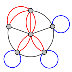
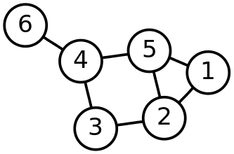
A one-dimensional simplicial complex is the same thing as a graph. The one-dimensional simplices of any simplicial complex are called edges, the two-dimensional simplices are called triangles and the three-dimensional ones are called tetrahedra. The picture below shows a graph with $P=\{1,2,3,4,5,6\}$ and seven edges.

graph

A one-dimensional simplicial complex $\mathcal{S}$ (a graph) can be viewed as a special one-dimensional cell complex $M$ (i.e. a special multigraph). The oriented edges of $M$ is the set of ordered pairs $(i,j)$ with $\{i,j\}\in \mathcal{S}^1$ and the maps $s,d,\rho$ are defined by

\begin{align*}s((i,j))&:=i\\ d((i,j))&:=j \\ \rho((i,j))&:=(j,i).\end{align*}

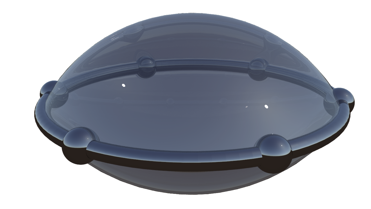
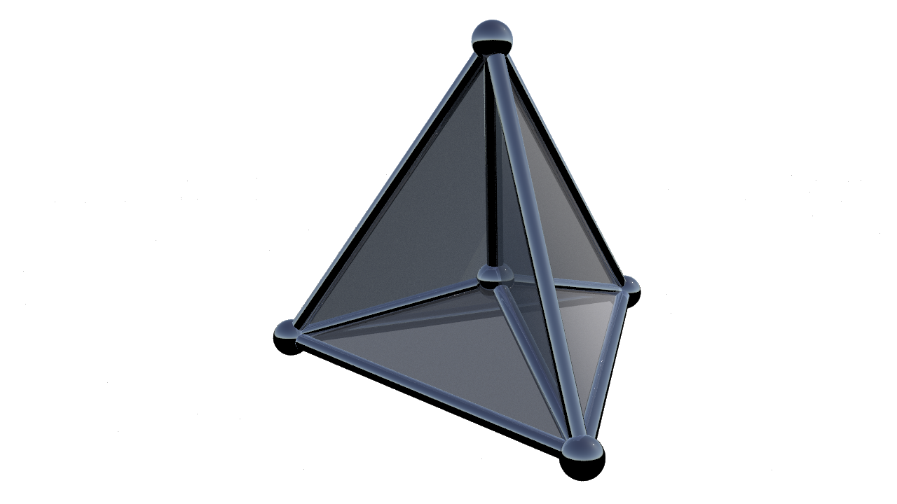
Similarly, a two-dimensional simplicial complex can be viewed as a special two-dimensional cell complex. The cell-complex below from the last post arises in this way from a two-dimensional simplicial complex with five points, ten edges and six triangles.

tet-cone-simple

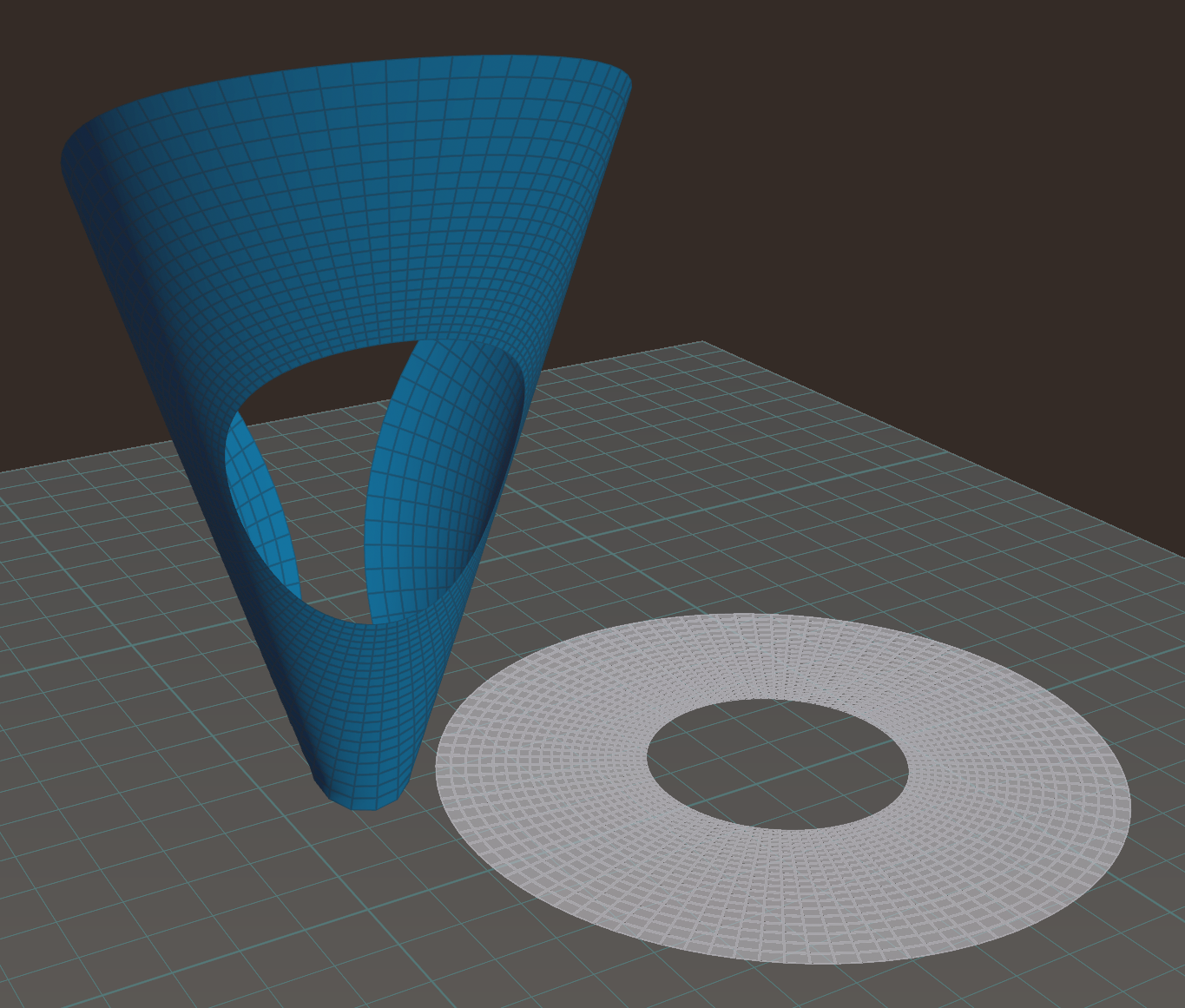
We have not really discussed this, but a two-dimensional cell complex describes a unique topological space. The same holds for general simplicial complexes. However, simplicial complexes are much more powerful for the discrete modeling of physical objects for the following reason: The topological space described by a combinatorial simplicial complex comes with a canonical piecewise affine structure. We now elaborate what this means.

Let $\mathcal{S}$ be a simplicial complex with point set $P$. Define then the piecewise affine space $C(\mathcal{S})$ corresponding to $\mathcal{S}$ as the set of all functions $f:P\to \mathbb{R}$ such that  $f(i)\geq 0$ for all $i\in P$,

$$\sum_{i\in P}\, f(i)=1$$

and

$$\big\{ \,i\in P \,\,\,\big|\,\,\, f(i)\neq 0\,\big\} \in \mathcal{S}.$$

For each simplex $S\in \mathcal{S}$ we define an affine space

$$\mathcal{A}_S:= \bigg\{\, g: P\to \mathbb{R} \,\,\,\bigg|\,\,\,\sum_{i\in P} g(i)=1\mbox{   and   }i\notin S \implies g(i)=0 \,\bigg\}$$

The vector space corresponding to the affine space $\mathcal{A}_S$ is

$$V_S:= \bigg\{\, g: P\to \mathbb{R} \,\,\,\bigg|\,\,\,\sum_{p\in P} g(i)=0\mbox{   and   }i\notin S \implies g(i)=0 \,\bigg\}$$

and each $\mathcal{A}_S$ is spanned by the simplex

$$\Sigma_S:=\big\{\, g\in\mathcal{A}_{S} \,\,\,\big|\,\,\,g(i)\geq 0 \mbox{   for all   } i\in P \,\big\}.$$

The whole space  $C(\mathcal{S})$ is the disjoined union of all the interiors (within $\mathcal{A}_S$) of the simplices $\Sigma_S$ for $S\in \mathcal{S}$. If $S\in \mathcal{S}$ and $T\subset S$ then $\mathcal{A}_T$ is an affine subspace of $\mathcal{A}_S$. Similarly, we also have $\Sigma_T \subset \Sigma_S$ in this case.

Each point $i\in P$ corresponds to a particular element $\delta_i\in C(\mathcal{S})$ defined by $\delta_i(j)=1$ for $j=i$ and $\delta_i(j)=0$ otherwise. We have $\mathcal{A}_{\{p\}}=\Sigma_{\{i\}}=\{\delta_i\}$. The main property that makes simplicial complexes useful for physical modeling is the following easy-to-prove

Theorem: Let $\mathcal{S}$ be a simplicial complex with point set $P$ and let  $f: P \to V$ be a map into any vector space $V$. Then there is a unique map

$$\hat{f}:C(\mathcal{S})\to V$$

whose restriction to each simplex $\Sigma_S$ is affine and which extends $f$ in the sense that for all $i\in P$ we have

$$\hat{f}(\delta_i)=f(i).$$

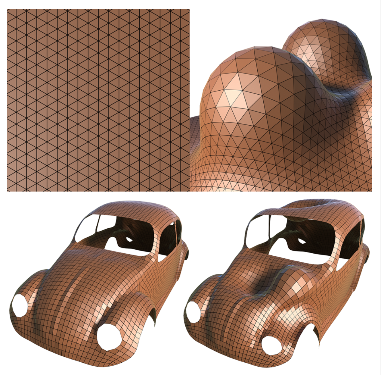
In particular, if we have a two-dimensional simplicial complex and are given a position in $\mathbb{R}^3$ for each of its points, it is clear how to fill in the triangles, for example in order to render them.

Posted in Lecture | Leave a comment