Laplace Operator

Let $M= \left(V, E, F \right)$ be an oriented triangulated surface without boundary and $p:V \rightarrow \mathbb{R}^3$ a realization. In earlier lectures we considered the space of piecewise linear functions on $M$:
\[W_{PL}:=\left\{ \tilde{f} :M\rightarrow \mathbb{R} \, \big \vert \,\left. \tilde{f}\right|_{\sigma} \mbox{ is affine for all } \sigma \in F \right\}.\]
A basis of $W_{PL}$ is given by : $\phi_i \in W_{PL}$ defined by $\phi_i(p_j) = \delta_{ij},$ an  interpolation map is defined by:
\begin{align*} \mbox{int}_{PL} : \mathbb{R}^{V}  & \rightarrow W_{PL}, \\
f  & \mapsto \tilde{f} = \sum_{i \in V} f_i \phi_i.
\end{align*}

graph phi

The graph of $\phi_i$

For some purposes piecewise constant function are more convenient then piecewise linear ones, therefore, we introduce a new function space on $M$ that consists of piecewise constant functions. In order to do that we assign a domain to each vertex:
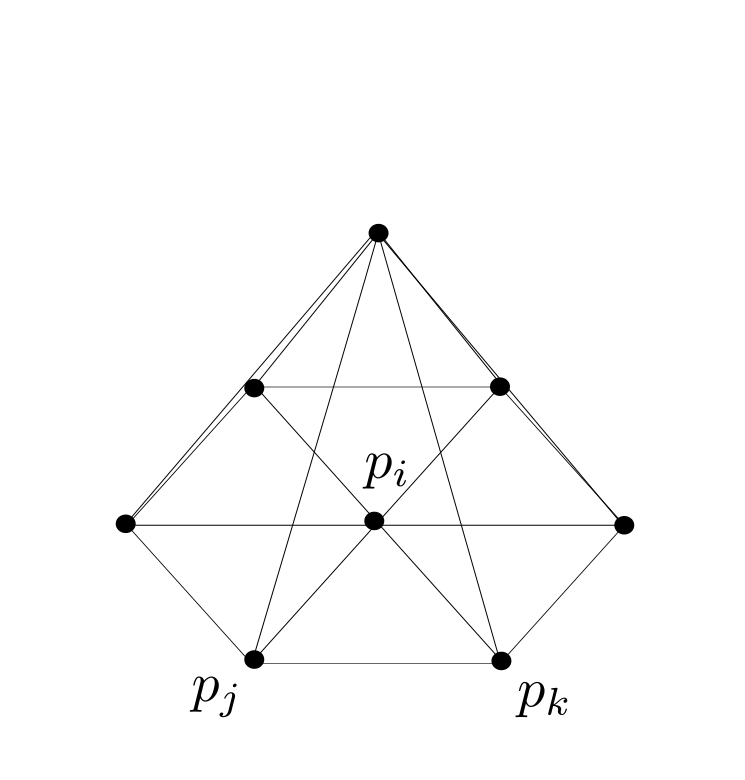
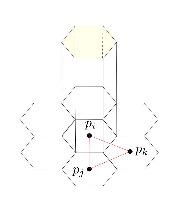
For every edge $e_{ij} \in E$ the center is given by $S_{ij}= \frac{1}{2}\left( p_i + p_j \right)$ analog  for every triangle $\sigma = \{i,j,k\} \in F$ the center of mass is defined as $S_{ijk} = \frac{1}{3} \left( p_i + p_j + p_k\right) $.

trianglemasscenter

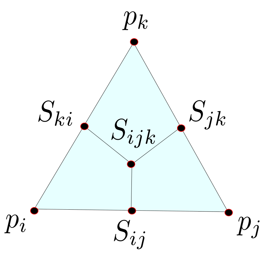
If we connect the center of the edges with the center of mass the triangle is divided into three parts with equal area. Now we can assign to each vertex $p_i$ the parts of the adjacent triangles that contain $p_i$ and denote it with $D_i$.

pointarea

The domain $D_i$ (gray colored) associated to the vertex $p_i$

For the area of $D_i$ we obtain:
\[A_i := \frac{1}{3} \sum_{ \sigma = \{i,j,k\} \in F} A_{\sigma}. \]

The space of piecewise constant functions is defined in the following way:
\[W_{PC}:= \left\{\hat{f} :M \rightarrow \mathbb{R} \, \big \vert \, \left. \hat{f}\right|_{D_i} \mbox{ is constant for all } i \in V \right\}.\]
Also on $W_{PC}$ we have a canonical basis $\Psi_i \in W_{PC}$ defined by $\Psi_i(p_j) = \delta_{ij} $ and an interpolation map:
\begin{align*} \mbox{int}_{PC} : \mathbb{R}^{V}  & \rightarrow W_{PC}, \\
f  & \mapsto \hat{f} = \sum_{i \in V} f_i \Psi_i.
\end{align*}

graph psi

Graph of $\Psi_i$

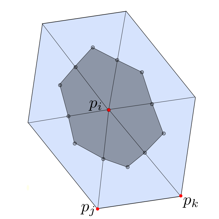
There is a similar construction that assigns to each vertex an face and works purely combinatorial: For a triangulated $M$ surface one can define its discrete dual surface $M^{\ast}=\left( V^{\ast},E^{\ast},F^{\ast}\right)$. The faces of $M$ correspond to the vertices of $M^{\ast}$ and the vertices of $M$ to the faces of $M^{\ast}$. The set of edges stays the same. Two vertices in $M^{\ast}$ are connected by  an edge if the corresponding faces in $M$ are adjacent. For more informations see here.

dualsurface

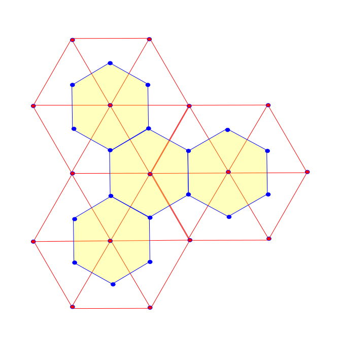
A piece of an triangulated surface $M$ and its dual $M^{\ast}$. The red vertices and edges belong to $M$ and the blues ones to $M^{\ast}$.

Since in general it is not easy to compute the area of the dual faces with the metric of the original one, we used the above construction of the $D_i$’s to define $W_{PC}$. On $W_{PL}$ we defined the usual scalar product $ \langle\!\langle \tilde{f}, \tilde{g} \rangle\!\rangle_{PL}  := \int_M \tilde{f}\tilde{g}$ and computed the matrix $B$ representing it with respect to the basis $\left\{ \phi_1,\ldots \phi_N \right\},$ i.e. $b_{ij}:=\langle\!\langle\phi_i, \phi_j \rangle\!\rangle_{PL}.$ This gave us a scalar product on $\mathbb{R}^V$:

\[\langle\!\langle f, g \rangle\!\rangle_{PL} =  f^tBg = \sum_{i,j \in V} f_i g_j b_{ij}.\]

On the same way we define an scalarproduct on $W_{PC}$:
\begin{align*}\langle\!\langle\cdot, \cdot \rangle\!\rangle_{PC} &: W_{PC}\times W_{PC} \rightarrow \mathbb{R}, \\ \langle\!\langle \hat{f}, \hat{g} \rangle\!\rangle_{PC} & := \int_M\hat{f}\hat{g}.\end{align*}
The matrix $A$ representing it with respect to the basis  $\left\{ \Psi_1,\ldots \Psi_N \right\}$ is a diagonal matrix since:
\[a_{ij}:=\langle\!\langle\Psi_i, \Psi_j \rangle\!\rangle_{PC}\ = \int_M \Psi_i \Psi_j = A_i \delta_{ij}.\]
This gives us a new  scalar product on $\mathbb{R}^V:$
\[\langle\!\langle f, g \rangle\!\rangle_{PC} :=  f^tAg = \sum_{i \in V} f_i g_i a_{ii}.\]
Note that the basis $\left\{ \Psi_1,\ldots \Psi_N \right\}$ is orthogonal with respect to $\langle\!\langle \cdot, \cdot \rangle\!\rangle_{PC}$, while the same is not true for $\left\{ \phi_1,\ldots \phi_N \right\}$ with respect to $\langle\!\langle \cdot, \cdot \rangle\!\rangle_{PL}$.
Now we have two scalar products on $\mathbb{R}^V$ one represented by a symmetric positive definite matrix $B$ and one by a positive definite diagonal one $A$.
Our aim is to define a discrete laplace operator $\Delta:\mathbb{R}^V  \rightarrow \mathbb{R}^V$ analog to the smooth laplacian we discussed earlier. We will see that the discrtelaplacian depends on the choice of scalarproduct.
On a smooth surface $M$ we have:
\[\langle\!\langle \Delta f, g \rangle\!\rangle = \int_M \Delta f g =\, – \int_M \langle \mbox{grad}\, f , \mbox{grad}\, g \rangle.\]
This identity should also be true in the discrete case and will serve us as definition for the discrete laplacian. We already defined the bilinear operator
\begin{align} L: \mathbb{R}^V \times \mathbb{R}^V & \rightarrow \mathbb{R},\\ f,g & \mapsto \, – \int_M \langle \mbox{grad}\, f , \mbox{grad}\, g \rangle ,\end{align}

and discussed the relation between  quadratic forms, symmetric bilinear maps and maps between dual spaces ( lecture: dirichlet energy 2 ).
\[\begin{array}{lcl} W_{PL} & \overset{E_D}{\longrightarrow}  & W_{PL}^{\ast} \\ \uparrow \mbox{interpol.} &  & \downarrow \mbox{interpol.}^{\ast} \\ \mathbb{R}^V & \overset{L}{\longrightarrow} & \mathbb{R}^{V\ast} \end{array}  \]
In the finite case the quadratic form, bilinear form and map between the dual spaces can all be represented by the same matrix $L$ .

For $f,g \in \mathbb{R}^V$ we have:
\[f^tLg = \,- \int_M \langle \mbox{grad}\, f , \mbox{grad}\, g \rangle\overset{!}{=} \int_M \Delta f g = \langle\!\langle \Delta f, g \rangle\!\rangle .\]
This gives us one laplace operator for each scalarproduct on $\mathbb{R}^V$:
\begin{align} f^tLg = \left\{ \begin{array} {cc} \left(\Delta_{PL} f\right)^tBg, \\ \left(\Delta_{PC} f\right)^tAg,\end{array} \right. \\ \Rightarrow \left\{ \begin{array} {cc} \Delta_{PL} = \left(LB^{-1} \right)^t = B^{-1}L , \\ \Delta_{PC} = \left(LA^{-1} \right)^t = A^{-1}L. \end{array} \right. \end{align}

In general it is complicated and expensive to compute $B^{-1}$, such that it is much easier to use $\Delta_{PC}$ instead of $\Delta_{PL}$. Witch of the laplacians one has to choose depends on the nature of the problem.

One famous problem form physics and geometry is the Poisson problem:
Given $\rho \in \mathbb{R}^V$ find $u \in \mathbb{R}^V$ such that:
\[\Delta \,u = -\rho.\]
For Poisson problems both laplacians can be used since:

\[\Delta_{PL} u = \left(LB^{-1} \right)^t u = \,- \rho \Leftrightarrow Lu = -B\rho. \]

Example: Suppose $M$ consists of an uniform conducting material and $\rho: M \rightarrow \mathbb{R}$ is a charge density. For the electric field $E$ on $M$ there holds:
\[\mbox{div} E = \rho,\]
and for the potential $u: M \rightarrow \mathbb{R}$ we have
\[E=-\mbox{grad}\, u.\]Taking this together we have to solve:
\[\Delta \,u = -\rho,\]
in order to determine the potential for a given density.
In this setting piecewise constant functions are much more convenient to describe the charge density then piecewise linear ones. Therefore we use $\Delta_{PL} $ to solve this problem.

Posted in Lecture | Leave a comment

Dirichlet Energy

Let $M$ be a triangulated domain with the functionspace:
\[W_{PL}:=\bigl\{f:M\rightarrow\mathbb{R}\,\bigl\vert\bigr.\,\,\,\left. f\right|_{T_{\sigma}} \mbox{ is affine for all } \sigma \in \Sigma_2 \bigr\}.\]
On the interior of each triangle $T_{\sigma}$ in $M$ the gradient of a function $g \in W$ is well defined and constant. We will derive a nice formula to compute $\left. \mbox{grad}\;g \right|_{T_{\sigma}}$.

Theorem 1: Let $T \subset \mathbb{R}^2$ be a non degenerated triangle with vertices $p_i,p_j,p_k$ and edges $e_i :=p_k-p_j$, $e_j :=p_i-p_k$, $e_k :=p_j-p_i$. For an affine function $g:T\rightarrow \mathbb{R}$ we define $g_i:=g(p_i)$, $g_j:=g(p_j)$, $g_k:=g(p_k)$. Then there holds:
\[\mbox{grad}\, g = \frac{1}{2A}J\bigl( g_i e_i+g_j e_j+ g_k e_k\bigr),\]
where $A:=\frac{1}{2}\mbox{det}(e_i,e_j) = \frac{1}{2} \langle Je_i,e_j \rangle=\frac{1}{2}\langle Je_j,e_k \rangle=\frac{1}{2}\langle Je_k,e_i \rangle,$ denotes the area of $T$ and $J$ the usual $90$ degree rotation in the plan.

Proof: In order to compute $\mbox{grad}\, g$ consider the curvepath6075-9
\begin{align*} & \gamma : [0,1] \rightarrow \mathbb{R}^2,\\ & \gamma(t)  :=p_j + te_i. \end{align*}
The composition of $g$ and $\gamma$ is given by: $\left( g\circ \gamma\right)(t) = g_j + t\left( g_k – g_j\right)$. Taking the derivative direct and with respect to the product rule we get:
\[g_k -g_j = \left( g\circ \gamma\right)'(t) = g’\left(\gamma(t)\right) \cdot\gamma'(t) = \langle \mbox{grad} \, g, \gamma'(t) \rangle = \langle \mbox{grad} \, g,e_i \rangle. \]
On the other hand we have:
\begin{align*}\bigl\langle\frac{1}{2A}J\left( g_i e_i+g_j e_j+ g_k e_k\right),e_i \bigr\rangle & = \frac{1}{2A} \bigl(g_i \underbrace{\langle Je_i,e_i\rangle }_{=0} + g_j \underbrace{\langle Je_j,e_i\rangle}_{=-2A} + g_k \underbrace{\langle Je_k,e_i\rangle}_{= 2A}\bigr) \\ &= g_k -g_j.\end{align*}
And therfore:
\[\bigl\langle\frac{1}{2A}J\left( g_i e_i+g_j e_j+ g_k e_k\right),e_i \bigr\rangle = \bigl\langle \mbox{grad} \, g,e_i \bigr\rangle.\]
A cyclic permutation of $i,j,k$  gives us:
\[\bigl\langle\frac{1}{2A}J\left( g_i e_i+g_j e_j+ g_k e_k\right),e_j \bigr\rangle = \bigl\langle \mbox{grad} \, g,e_j \bigr\rangle,\]
and we obtain the desired result \[\mbox{grad}\, g = \frac{1}{2A}J\bigl( g_i e_i+g_j e_j+ g_k e_k\bigr).\]

$\square$

Definition: For $g \in W_{PL}$ the Dirichlet energy is defined as:
\[E_D(g) := \frac{1}{2} \int_M \left| \mbox{grad} \, g \right|^2.\]

Theorem 2: We use the same notation as in theorem 1. Additionally let $\alpha_i,\,\alpha_j,\, \alpha_k$ denote the angles of the triangle at the vertices $p_i, \, p_j, \, p_k$ respectively. Then there holds:
\[ \int_T \left| \mbox{grad} \, g \right|^2 = \frac{1}{2}\bigl( \cot (\alpha_i) (g_j-g_k) ^2 + \cot (\alpha_j) (g_k-g_i) ^2 + \cot (\alpha_k) (g_i-g_j) ^2\bigr).\]

Proof: \begin{multline}\int_T \left| \mbox{grad} \, g \right|^2 = \int_T \langle \frac{1}{2A}J\left( g_i e_i+g_j e_j+ g_k e_k\right), \frac{1}{2A}J\left( g_i e_i+g_j e_j+ g_k e_k\right) \rangle \\ =\frac{A}{4 A^2} \Bigl(\Bigr. g_i^2 |e_i|^2 +  g_j^2 |e_j|^2 + g_k^2 |e_k|^2 + 2g_ig_j \langle e_i,e_j \rangle + 2g_jg_j \langle e_j,e_k \rangle + 2g_kg_i \langle e_k,e_i \rangle \Bigl)\Bigr..  \end{multline}
On the other hand we have:
\begin{align}\frac{-1}{4A} \bigl(\bigr. \left( g_i -g_j\right)^2 & \langle e_i, e_j \rangle +\left( g_j -g_k\right)^2 \langle e_j, e_k \rangle +\left( g_k -g_i\right)^2 \langle e_k, e_i \rangle \bigl)\bigr. \\ &= \frac{-1}{4A} \bigl(\bigr. g_i^2 \langle e_i,\underbrace{e_j + e_k}_{= – e_i}\rangle -2g_ig_j\langle e_i,e_j \rangle + g_j^2 \langle e_j, \underbrace{e_i + e_k}_{= – e_j}\rangle \\ &\quad\quad\quad -2g_kg_j\langle e_k,e_j \rangle +g_k^2 \langle e_k, \underbrace{e_j + e_i}_{=- e_k}\rangle -2g_ig_k\langle e_i,e_k \rangle \bigl)\bigr. \\ &= \frac{1}{4 A} \bigl(\bigr. g_i^2 |e_i|^2 +  g_j^2 |e_j|^2 + g_k^2 |e_k|^2 \\ &\quad\quad\quad+ 2g_ig_j \langle e_i,e_j \rangle + 2g_jg_j \langle e_j,e_k \rangle + 2g_kg_i \langle e_k,e_i \rangle \bigl)\bigr. \\ & = \int_T \left| \mbox{grad} \, g \right|^2.\end{align}
With \begin{align*}\langle e_i,e_j \rangle & = -\cos (\alpha_k) |e_i||e_j|,\\2A = \frac{1}{2}\mbox{det}(e_i,e_j) & = \frac{1}{2} \langle Je_i,e_j \rangle
= \sin(\alpha_k) |e_i||e_j|.\end{align*}
We have:
\[\cot(\alpha_k) = \frac{-\langle e_i,e_j \rangle}{2A}.\]
And therefore we obtain for the Dirichlet energy of $g$ on $T$:
\[ \int_T \left| \mbox{grad} \, g \right|^2 = \frac{1}{2}\bigl( \cot (\alpha_i) (g_j-g_k) ^2 + \cot (\alpha_j) (g_k-g_i) ^2 + \cot (\alpha_k) (g_i-g_j) ^2\bigr).\]

$\square$

Corollary: The Dirichlet energy of $g \in W_{PL}$ is given by :
\[E_D(g) = \frac{1}{4} \sum_{\sigma = \{i,j,k\} \in \Sigma_2}  \cot (\alpha_i) (g_j-g_k) ^2 + \cot (\alpha_j) (g_k-g_i) ^2 + \cot (\alpha_k) (g_i-g_j) ^2.\]

 2triangles

If $E:= \left\{ \{i,j\} \in \Sigma\right\}$ denotes the set of edges and $\tilde{E}:= \left\{ (i,j) \in V \times V\, \big \vert \{i,j\} \in \Sigma\right\}$ the set of oriented edges, we choose $\hat{E} \subset \tilde{E}$ such that:

1)  $E = \left\{ \{i,j\} \subset V \big \vert (i,j) \in \hat{E}\right\}$,
2)  $(i,j) \in \hat{E} \rightarrow (j,i) \notin \hat{E}.$

I.e. for every edges we choose oneoriented one. For every $(i,j) \in \hat{E}$ let $\alpha_{ij}$ denote the angle of the opposite vertex to the left and $\beta_{ij}$ the one the opposite vertex to the right. Then we can write the Derichlet energy in the following form:
\[E_D(g) = \frac{1}{4} \sum_{(i,j) \in \hat{E}} \left( \cot(\alpha_{ij}) + \cot{\beta_{ij}}\right) \left(g_i-g_j \right)^2, \]
where we set the cotangent weights zero if the corresponding vertex does not exist because $(i,j)$ is an boundary edge.

Posted in Lecture | Leave a comment

Tutorial 5: Holomorphic Null-Curves—Associated Family and Goursat transforms

Let \(M\subset \mathbb C\) be an open set and \(V\) a complex vector space with a non-degenerated complex-valued symmetric complex-bilinear form \(\langle.,.\rangle\). A null-curve is a map \(\gamma \colon M \to V\) such that\[\gamma^\ast\langle.,.\rangle = \langle d\gamma,d\gamma\rangle = 0\,.\]Unless explicitly stated differently \(\mathbb C^n\) is always equipped with its standard bilinear form\[\langle \psi,\psi\rangle = \sum_{i=1}^n \psi_i^2\,,\]which restricts to the standard inner product on \(\mathbb R^n\subset \mathbb C^n\).

Theorem. If \(\gamma\colon M \to \mathbb C^n\) is a holomorphic null-curve, then—away from the singular points of \(\gamma\)—the map \(f = \mathrm{Re}\,\gamma\) is a conformally immersed minimal surface.

Proof. Since \(\gamma\) is holomorphic, we have \(\gamma_y = i\gamma_x\). Thus we get \(\gamma_x = f_x -if_y\). The null-curve condition then yields\[0 = \langle \gamma_x,\gamma_x\rangle = |f_x|^2 – |f_y|^2 – 2i\langle f_x,f_y\rangle\]and thus \(|f_x|^2 = |f_y|^2\) and \(\langle f_x,f_y\rangle = 0\)—meaning that \(f\) is conformal. Moreover, as the real part of a holomorphic map, \(f\) is harmonic, which means that it is minimal. \(\square\)

Conversely, it is not hard to show that that—at least on a simply-connected domain \(M\)—each conformally immersed minimal surface comes from such a holomorphic null-curve. Moreover, the notion of a holomorphic null-curve extends in the obvious way to maps from a Riemann surface into a complex manifold with complex-bilinear fiber product.

Now let us equip \(\mathbb C^5\) with another bilinear form: For \(\psi=(\psi_1,\ldots,\psi_5) \in \mathbb C^5\), we set\[\langle\psi,\psi\rangle = \psi_1^2 +\psi_2^2 +\psi_3^2 -\psi_4\psi_5\,.\]This bilinear form restricts to an inner product of signature \((++++-)\) on \(\mathbb R^n\) and \(\mathcal L = \{\psi \in \mathbb C^5\setminus \{0\} \mid |\psi|^2 = 0\}\) is its complexified light-cone. Let furthermore \(\mathcal L_\ast\) denote the set of vectors in \(\mathcal L\) with non-vanishing last component,\[\mathcal L_\ast = \{\psi\in \mathcal L \mid \psi_5 \neq 0\} = \mathcal L \setminus (\mathbb C^4\times \{0\})\,.\]We define two maps:\[\sigma \colon  \mathcal L_\ast \to\mathbb C^3,\quad \psi\mapsto \tfrac{1}{\psi_5}(\psi_1,\psi_2,\psi_3)\]and\[\tau \colon \mathbb C^3 \to \mathcal L_\ast,\quad x\mapsto (x,|x|^2,1)\,.\]One easily checks the following identities: Let \(\beta \colon \mathbb C^5 \to \mathbb C\) denote the projection to the 5th component, \(\beta(\psi) = \psi_5\), then \[\sigma\circ\tau = \mathrm{id}_{\mathbb C^3},\quad \tau\circ \sigma = \tfrac{1}{\beta}\mathrm{id}_{\mathcal L_\ast}\,.\]

Obviously the maps \(\sigma\) and \(\tau\) both preserve holomorphicity: If \(\varphi\colon M\to \mathcal L\) is holomorphic, then \(\gamma = \sigma\circ \varphi\) is meromorphic (holomorphic up to isolated points—the points for which \(\varphi\) hits \(\mathbb C^4\times\{0\}\)—where \(\gamma\) has poles). Conversely, any meromorphic \(\gamma\) appears from such a holomorphic \(\varphi\).

Lemma. \(\sigma^\ast \langle.,.\rangle = \beta^{-2}\langle.,.\rangle\) and \(\tau^\ast\langle.,.\rangle = \langle.,.\rangle\).

Proof.  If \(\dot x \in T_x \mathbb C^3\), we have \(d\tau(\dot x) = (\dot x, 2\langle \dot x,x\rangle, 0)\). Thus \(|d\tau(\dot x)|^2 = |\dot x|^2\) and hence \(\tau^\ast\langle.,.\rangle\). Thus we get \[\sigma^\ast\langle.,.\rangle =\sigma^\ast\tau^\ast\langle.,.\rangle = (\tau\circ\sigma)^\ast\langle.,.\rangle\,.\]Now, if \(\dot\psi \in T_\psi \mathcal L_\ast\), we have \(d(\tau\circ \sigma)(\dot \psi) = d(\tfrac{1}{\beta})(\dot\psi) \psi +\tfrac{1}{\beta}\dot \psi\). From \(|\psi|^2=0\), we also get \(\langle\psi,\dot\psi\rangle = 0\) and thus\[|d\sigma(\dot \psi)|^2=|d(\tau\circ \sigma)(\dot \psi)|^2 = \langle d(\tfrac{1}{\beta})(\dot\psi) \psi+\tfrac{1}{\beta}\dot \psi,d(\tfrac{1}{\beta})(\dot\psi)\psi+\tfrac{1}{\beta}\dot \psi\rangle = \tfrac{1}{\beta^2}\langle \dot\psi,\dot\psi\rangle\,.\]Hence \(\sigma^\ast\langle.,.\rangle = \beta^{-2}\langle.,.\rangle\). \(\square\)

Corollary. \(\sigma\) and \(\tau\) both preserve null-curves.

So we have seen that conformally immersed minimal surfaces in \(\mathbb R^3\) can be identified with null-curves in \(\mathbb C^3\) or \(\mathcal L\). Thus, if we find families of null-curves, we find families of minimal surfaces. An obvious such family is obtained by the action of \(\mathbb S^1\) on the complex vector space—this yields the so called associated family.

Lemma. If \(\varphi\colon M \to V\) is a holomorphic null-curve and \(c\in \mathbb S^1\subset\mathbb C\), then \(\varphi_c = c\varphi\) is a also a holomorphic null-curve.

Proof. We have \(d\varphi_c = c\, d\varphi\). Thus \(|\varphi_c|^2 = c^2|\varphi|^2=0\), i.e. \(\varphi_c\) is a null-curve. Since scalar multiplication by a constant is complex linear, holomorphicity is preserved as well. \(\square\)

The Kusner surfaces are obtained as the real part of the \(\mathbb C^3\)-valued meromorphic curve\[\gamma = \frac{i}{z^{2p}-1+rz^p}\Bigl(z^{2p-1} – z, -i(z^{2p-1} + z), \tfrac{p-1}{p}(z^{2p} +1)\Bigr)\,.\]where \(p\in \mathbb N\), \(r = 2\sqrt{2p-1}/(p-1)\) and \(z \colon \mathbb S^2 \to \mathbb C\) denotes the stereographic projection. One checks that \(\gamma\) is a null-curve. By the lemma above we can easily visualize its associated family by a slight modification of the last exercise.

Another source of families is the group of complex linear transformations that preserve the bilinear form: For \(V\) complex vector space with non-degenerate bilinear form \(\langle.,.\rangle\), then\[O(V) = \{A\in\mathrm{GL}(V)\mid \langle A\psi,A\tilde\psi\rangle = \langle\psi,\tilde\psi\rangle\quad \forall \psi,\tilde\psi\in V\}\,.\]The proof of the next lemma is almost identical to the last one. We omit it.

Lemma. Let \(\varphi\colon M \to V\) be a holomorphic null-curve, \(A\in O(V)\), then \(\tilde\varphi :=A\varphi\) is also a holomorphic null-curve.

We want to apply this to the Kusner surfaces. Therefore we first construct a lift \(\varphi\colon M \to \mathcal L\) of the Kusner null-curve \(\gamma\colon M \to \mathbb C^3\) above and then apply a linear transformation in \(\mathbb C^5\) preserving \(\mathcal L\). We make the following ansatz: For \(\rho\in \mathbb C\),\[\varphi =\Bigl(i(z^{2p-1} – z), (z^{2p-1} + z), i\tfrac{p-1}{p}(z^{2p} +1),\alpha(z),\rho(z^{2p}-1+rz^p)\Bigr)\,,\]where \(\alpha\) is a polynomial in \(z\) such that \begin{align*}\alpha(z) \rho(z^{2p}-1+rz^p) & = -(z^{2p-1} – z)^2 + (z^{2p-1} + z)^2 – (\tfrac{p-1}{p})^2(z^{2p} +1)^2\\ & =4z^{2p} – (\tfrac{p-1}{p})^2(z^{4p} +2z^{2p} +1)\\ & = – (\tfrac{p-1}{p})^2(z^{4p} +2(1-2\tfrac{p^2}{(p-1)^2})z^{2p} +1) \\& = – (\tfrac{p-1}{p})^2(z^{4p} +2\tfrac{1-2p-p^2}{(p-1)^2}z^{2p} +1)\,.\end{align*}On the other hand, we have\begin{align*}(z^{2p}-1 + rz^p)(z^{2p}-1 – rz^p) & = (z^{2p}-1)^2 – r^2z^{2p} \\ & = z^{4p} – (2+r^2)z^{2p} + 1 \\ & =z^{4p} – 2(1+2\tfrac{2p-1}{(p-1)^2})z^{2p} + 1\\ & = z^{4p} + 2\tfrac{1 – 2p – p^2}{(p-1)^2} z^{2p} + 1\end{align*}Thus we can set \(\rho = \tfrac{p-1}{p}\) and \(\alpha(z)=-\tfrac{p-1}{p}(z^{2p}-1 – rz^p)\) and obtain the following formula for the holomorphic null-curve:\[\varphi = \Bigl(i(z^{2p-1} – z), (z^{2p-1} + z), i\tfrac{p-1}{p}(z^{2p} +1),\tfrac{p-1}{p}(rz^p + (z^{2p}-1)),\tfrac{p-1}{p}(rz^p – (z^{2p}-1))\Bigr)\,.\]If we now apply a coordinate change \[e_1 \to e_1,\quad e_2\to e_2, \quad e_3\to e_3, \quad e_4 \to e_5 – e_4, \quad e_5 \to e_5 + e_4\,,\] then the bilinear form \(\langle.,.\rangle\) takes the form \[\langle \psi,\psi\rangle = \psi_1^2 + \psi_2^2 + \psi_3^2 + \psi_4^2 – \psi_5^2\] and is preserved by real rotation matrices mixing the first 4 components, as e.g. \[\begin{pmatrix}1 & 0 & 0 & 0 & 0 \\ 0 & \cos t & 0 & -\sin t & 0 \\0 & 0 & 1 & 0 & 0 \\ 0 & \sin t & 0 & \cos t & 0 \\ 0 & 0 & 0 & 0 & 1 \\\end{pmatrix},\quad t\in \mathbb R\,.\]If we apply it to the holomorphic null-curve which, after the coordinate change, looks as follows\[\tilde \varphi =\Bigl(i(z^{2p-1} – z), (z^{2p-1} + z), i\tfrac{p-1}{p}(z^{2p} +1),\tfrac{p-1}{p}(z^{2p}-1),\tfrac{p-1}{p}rz^p\Bigr)\]we obtain new a family of minimal surfaces. The \(\mathbb C^3\)-valued null-curve takes the form\[\gamma = \tfrac{1}{\tilde\varphi_5 – \tilde\varphi_4}(\tilde\varphi_1,\tilde\varphi_2,\tilde\varphi_3)\,.\]Here a sequence of members in the corresponding family:

The minimal surfaces have planar ends at the singularities. The pictures above show the part of the surface contained in a sphere of fixed radius. To achieve this, one can use the boolean sop node which allows to intersect a surface with the interior of a sphere. Make sure here that input A is treated as surface and input B is treated as volume.

Unfortunately, the node will produce artefacts unless we cut away vertices which are mapped to points whose magnitude is too large. Fortunately, there is a node to fix this. It is called Polycut and allows us to delete vertices on which a specified attribute exceeds a certain value (parameters should be set to Type: Points, Strategy:Remove, DetectEdgeChanges:Cut At Attribute Change). So we can just store the magnitude as an attribute on points (by a point wrangle node) and then use Polycut to remove all points which lie too far outside the ball we want to intersect the surface with.

Then intersect by a boolean node. There we select to generate a primitive group A Inside B so that we can delete everything else which which is not in this group using a blast node.

Homework (due 21 May): Wire up a network that visualizes (by two interactive parameters) the associated and an additional family of Kusner’s minimal surfaces.

Posted in Tutorial | Leave a comment

Tutorial 4: Boy’s Surface

The real projective plane \(\mathbb R\mathrm P^2\) is obtained by identifying the antipodal points of the a \(2\)-sphere \(\mathbb S^2\), i.e. \(\mathbb R\mathrm P^2 = \mathbb S^2/_\sim\) with equivalence relation given by \[ x\sim y \Leftrightarrow y = \pm x.\]
The real projective plane is a sphere with cross-cap – the fundamental polygon looks as follows:

The roman surface: It is known that there exists no embedding of \(\mathbb R\mathrm P^2\) into Euclidean \(3\)-space. Though it can be mapped to \(\mathbb R^3\) with self-intersection. An example is Steiner’s roman surface.

The corresponding map is given as follows:\[f\colon \mathbb R\mathrm P^2 \to \mathbb R^3, \quad [(x,y,z)]\mapsto \bigl(yz,zx,xy\bigr).\]

Cross-cap: Actually the roman surface is a projection of the Veronese surface into Euclidean \(3\)-space and as such a special case of a general construction method for non-orientable surfaces. Choosing a different projection we also obtain the cross cap from it:\[f\colon \mathbb R\mathrm P^2 \to \mathbb R^3, \quad [(x,y,z)]\mapsto \bigl(yz,zx,\tfrac{1}{2}(z^2-x^2)\bigr).\]

Boy’s surface: The maps above have singularities and it was not clear that an immersion exists until 1901. At that time Boy discovered an immersion which nowadays is known as Boy’s surface. It can be realized in different ways.

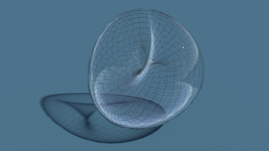
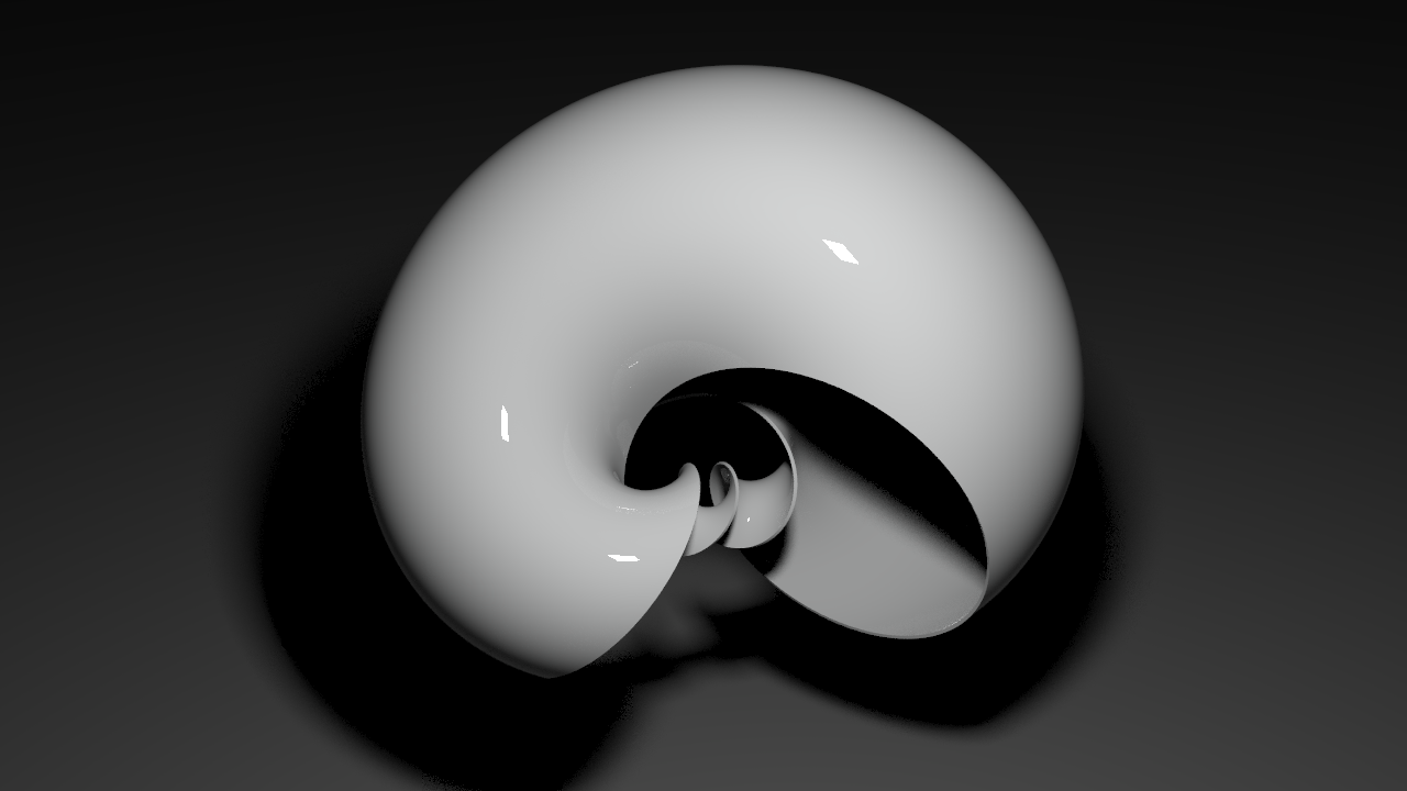
We will use the realization above due to Kusner and Bryant. It is especially beautiful in the sense that it is a critical point of the Willmore energy – a so called Willmore surface.

It is the inversion of a complete minimal surface with \(3\) ends and as a consequence rational, i.e. the immersion can be written down explicitly with rational functions. Actually it is known that all Willmore surfaces parametrized by spheres are obtained in this way.

This week your task is to visualize Boy’s surface. Its unorientability can be handled similarly to last week’s assignment: Everything will be done on \(\mathbb S^2\)—the orientation cover of \(\mathbb R\mathrm P^2\).

Kusner surfaces: Kusner gave an explicit formula for complete minimal surfaces with ends: Let \(p\in \mathbb N\) and \(r = 2\sqrt{2p-1}/(p-1)\). Let \(z \colon \mathbb S^2 \to \mathbb C\) be the stereographic projection. Then the immersion \(\mathbb S^2 \to \mathbb R^3\) is defined to be the real part of \[\Phi_p = \frac{i}{z^{2p}+rz^p-1}\Bigl(z^{2p-1} – z, -i(z^{2p-1} + z), \tfrac{p-1}{p}(z^{2p} +1)\Bigr).\]
The integer \(p\) controls the symmetry of the immersed surface. Below the surfaces for \(p=3,4,5\) and \(6\). Here we have cut out disks around the poles of \(\mathbb S^2\) for visualization purposes.

Finally we obtain Boy’s surface by a Möbius transformation of the Kusner surface with \(p=3\). The transformation is an inversion in the unit sphere with center \((0,0,h)\), \(h\neq 0\).

Implementation: The implementation is straight forward. The network could look as follows:

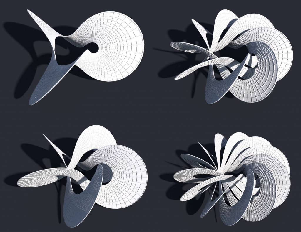
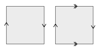
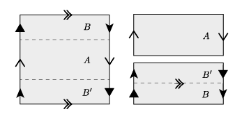
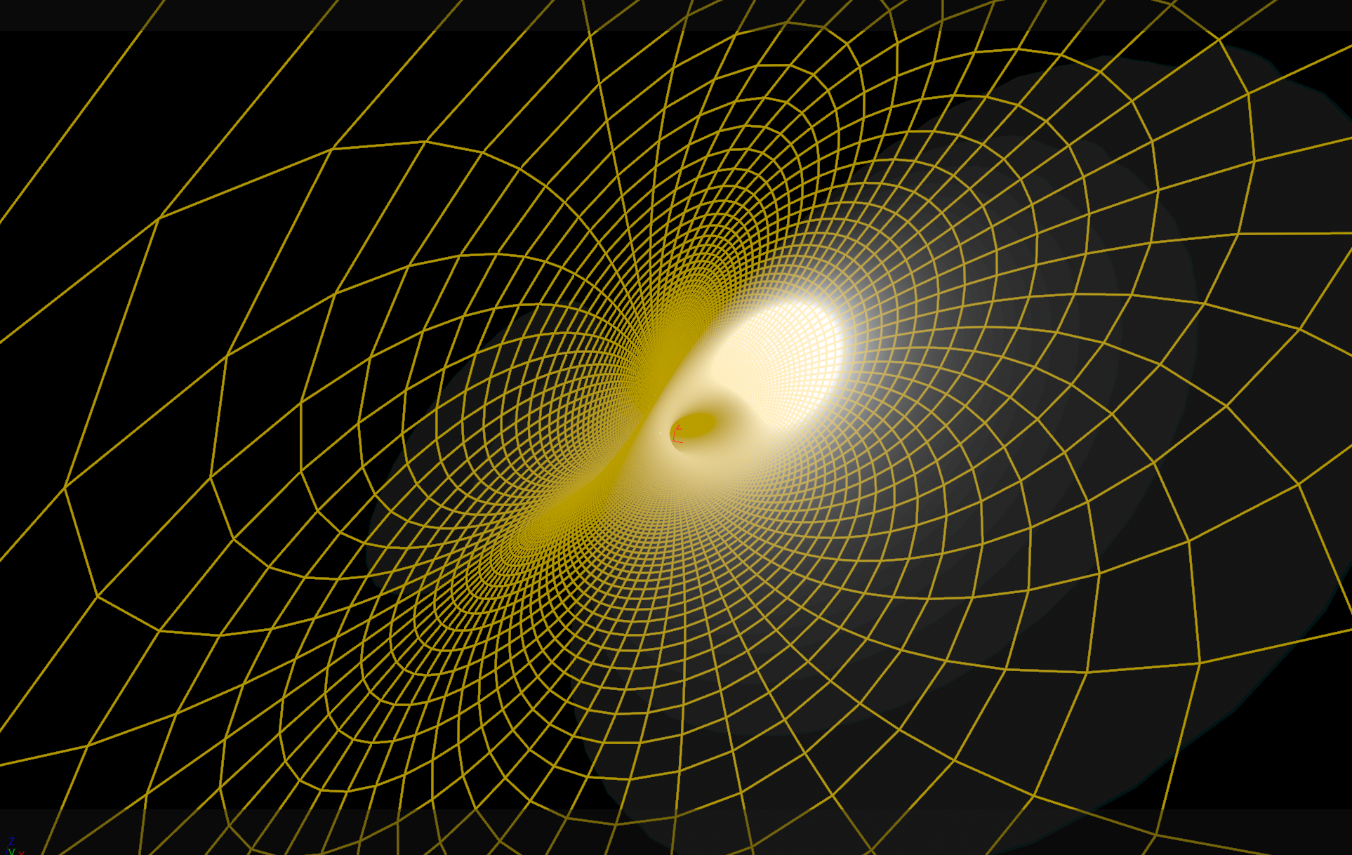
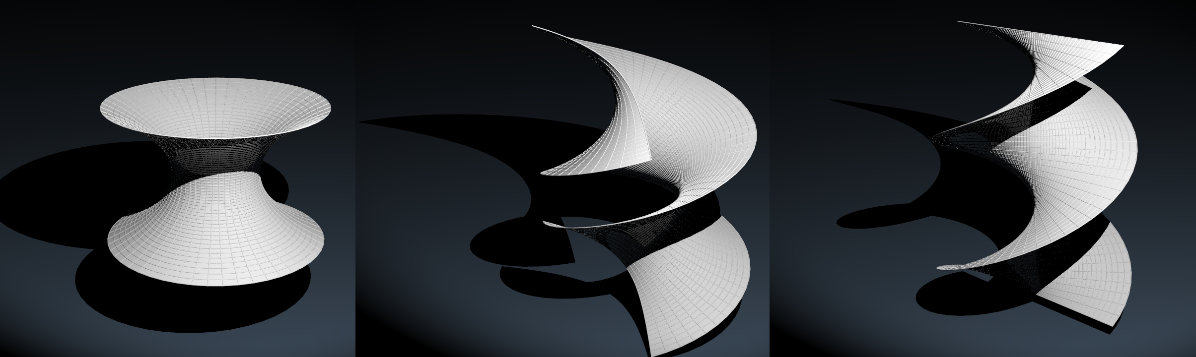
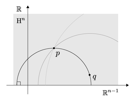
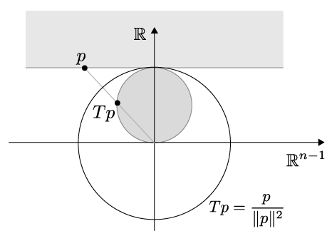
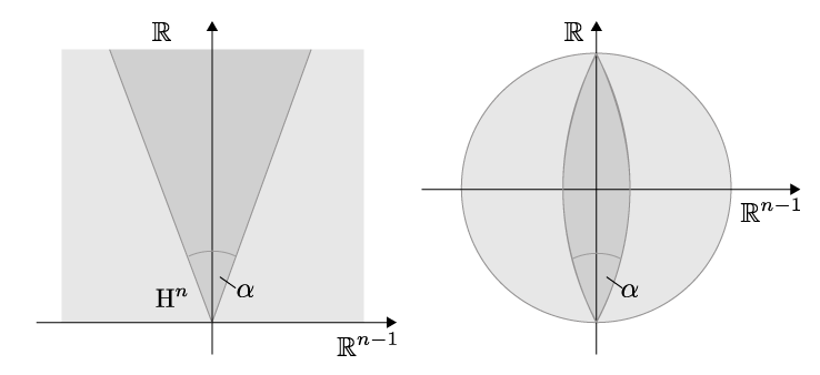
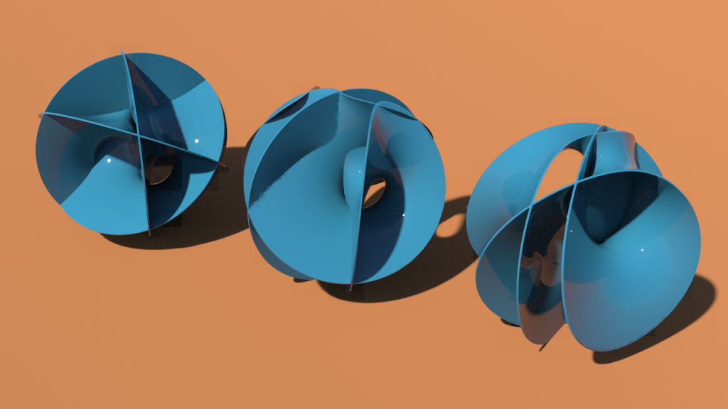
We start with a sphere, apply the stereographic projection (poinwrangle1), Kusner’s formula (pointwrangle2) and finally the inversion in the sphere (pointwrangle3).

The node subnet1 contains a small network that cuts off a cap from the north pole and a cap from the south pole of the sphere. This can be done by two clip nodes.

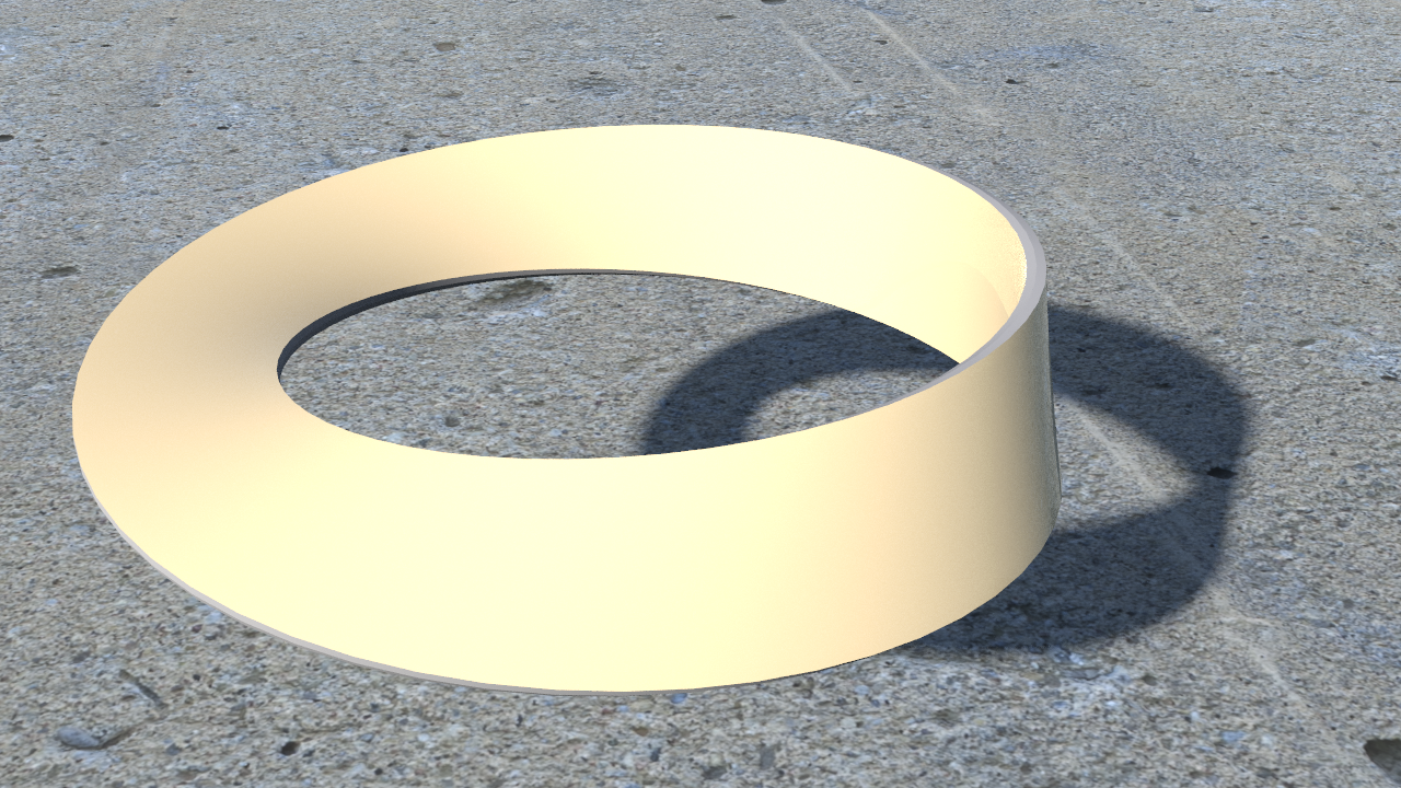
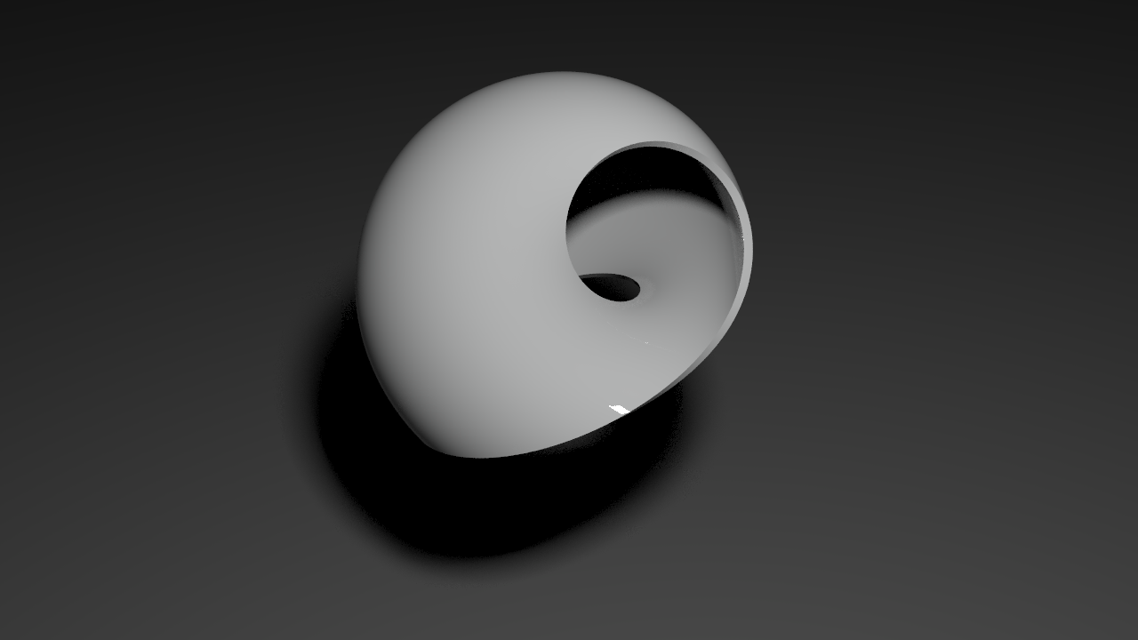
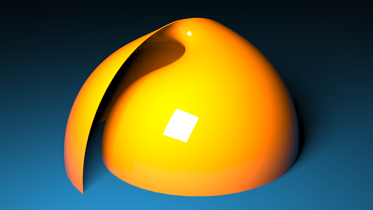
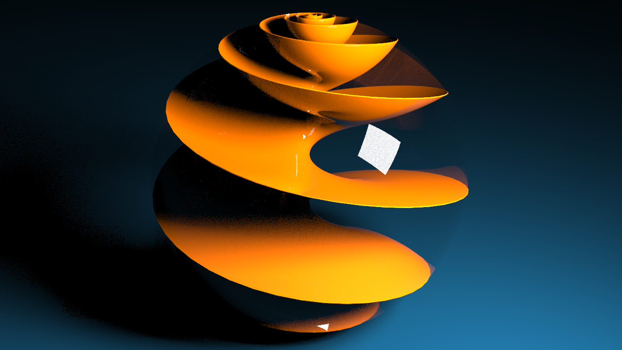
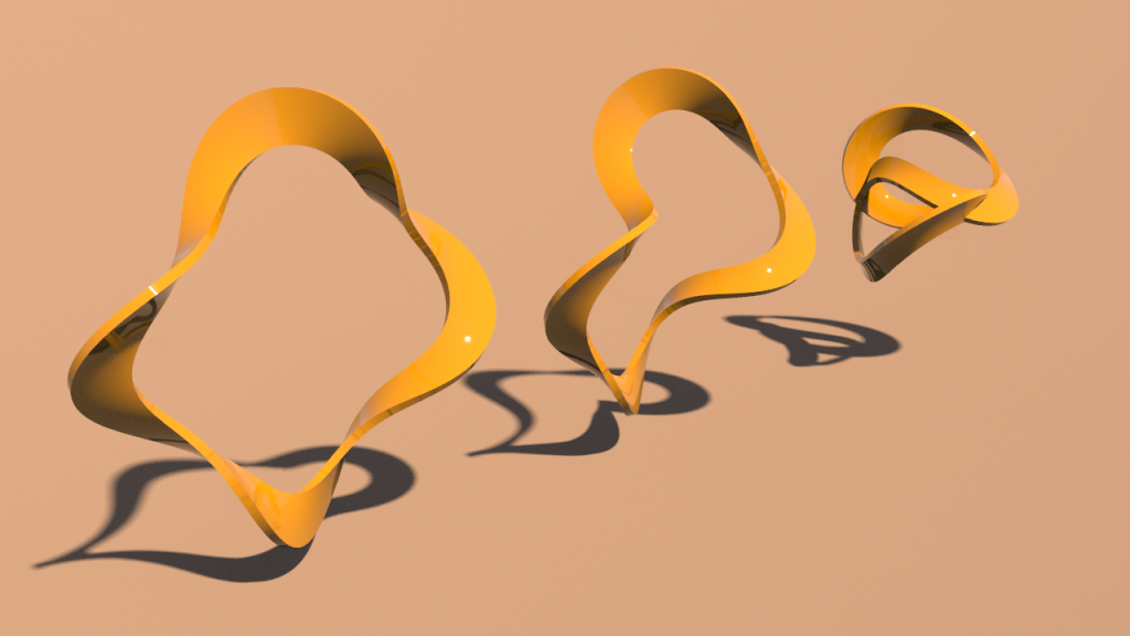
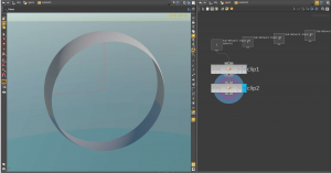
Cutting this holes symmetrically corresponds to cutting a disk from \(\mathbb R\mathrm P^2\). Thus the cylinder above is mapped to a Möbius strip on Boy’s surface.

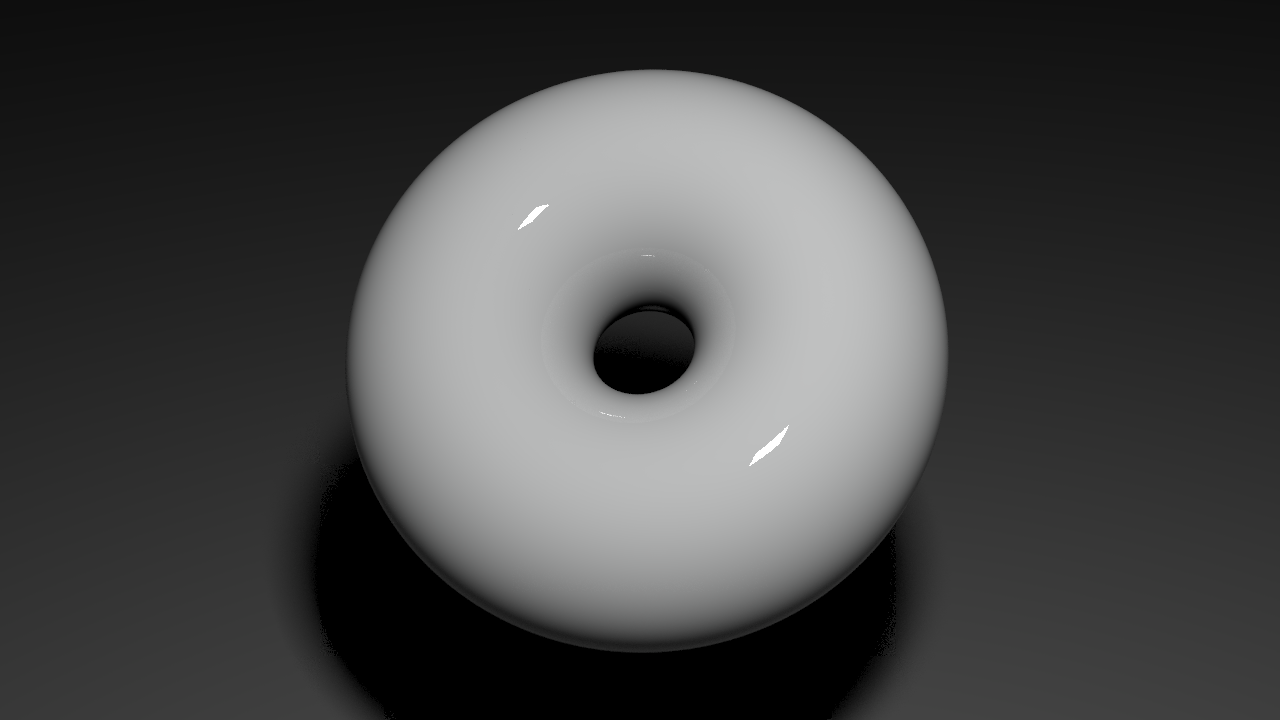
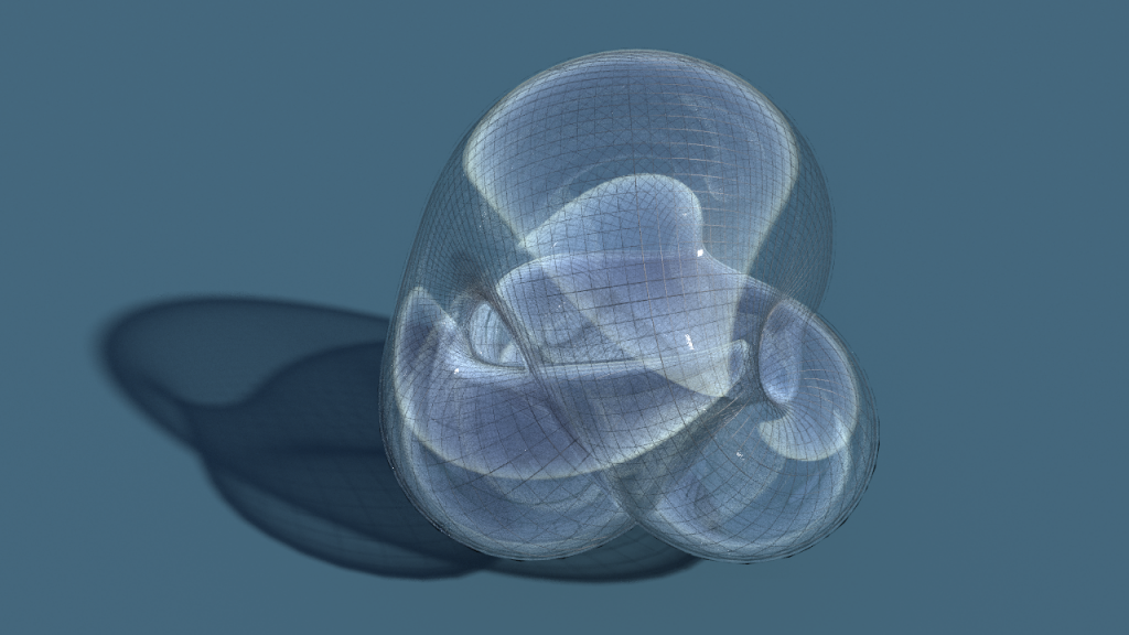
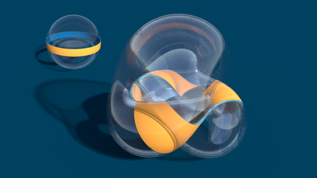
Though the surface is still quite hard to understand from the picture. One way to understand it better is to use a parameter for the width of the strip. Here a sequence for growing width.

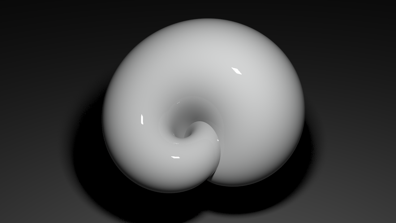
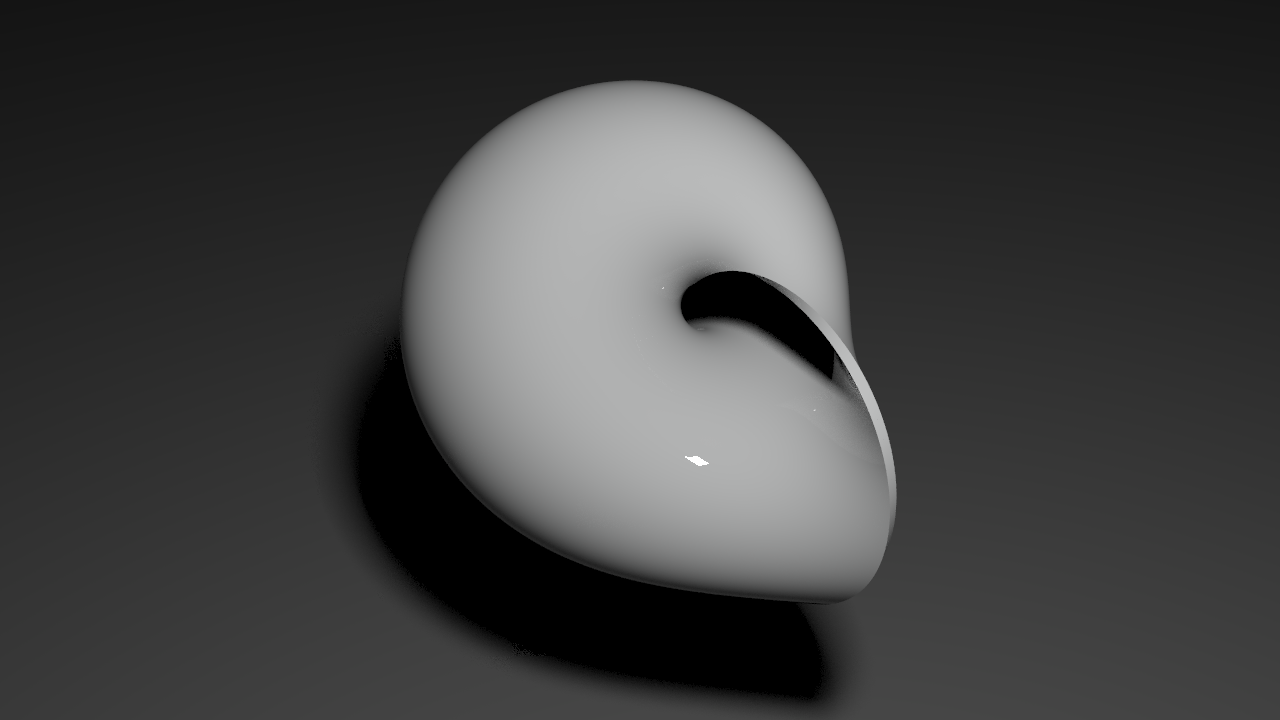
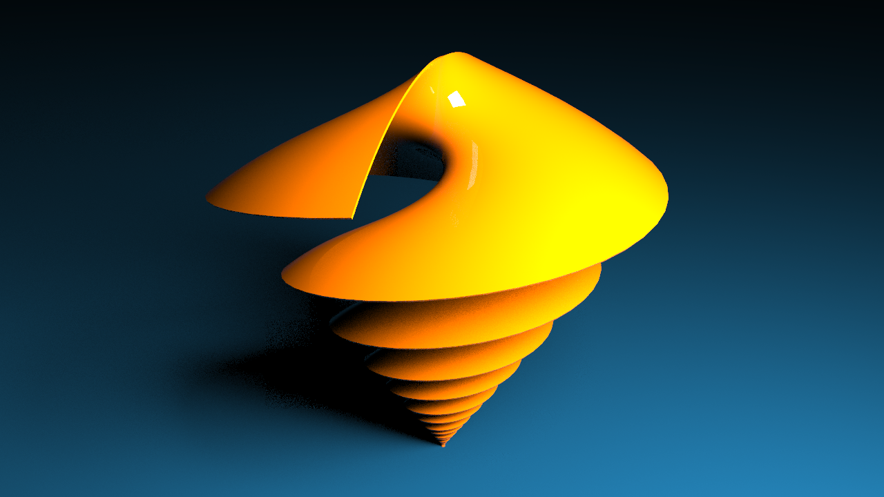
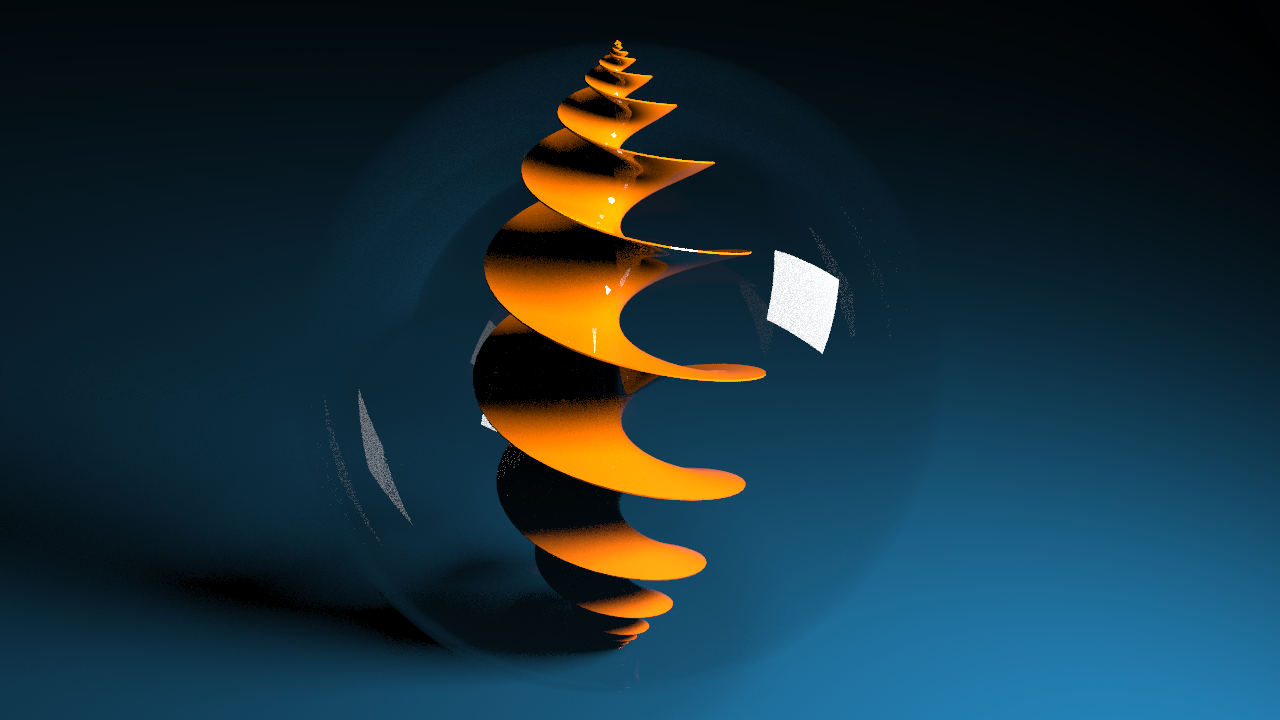
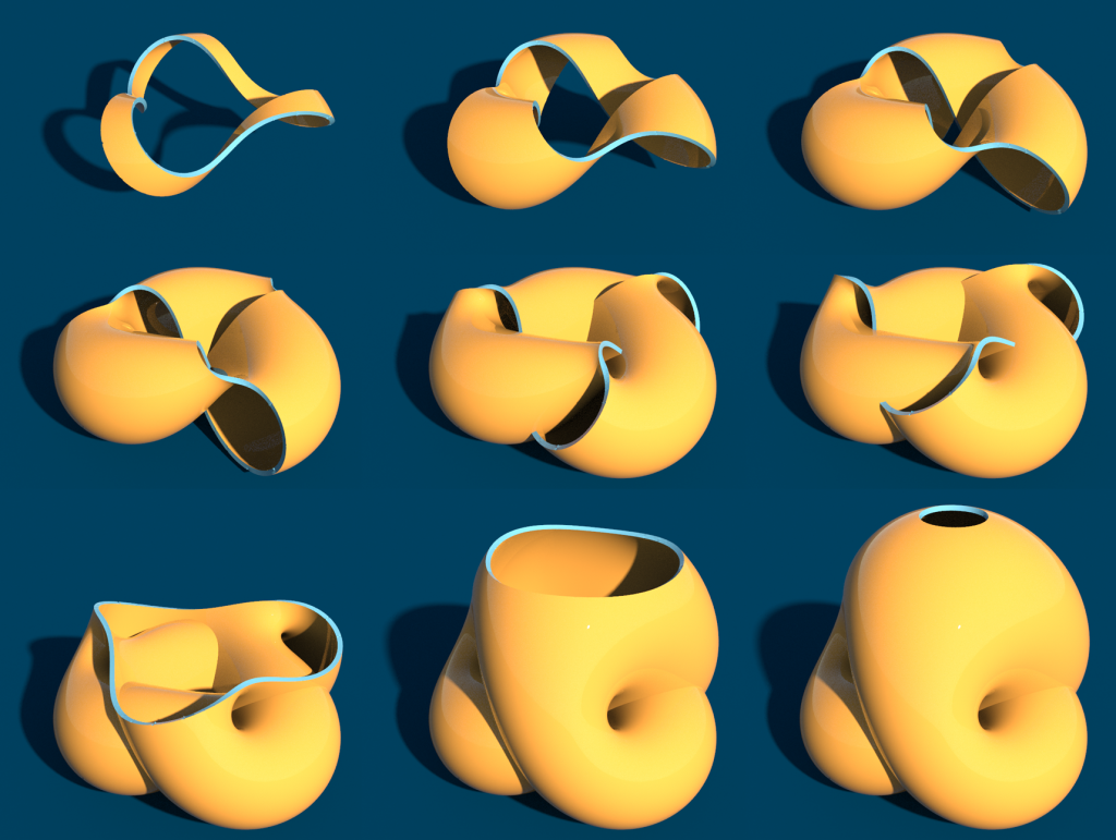
If we move the strip up and destroy the symmetry the two sheets of the covering become visible.

Note that a cell decomposition of \(\mathbb R\mathrm P^2\) is basically a cell decomposition of \(\mathbb S^2\) which is mapped by the antipodal map to itself. One way to obtain such a cell decomposition is by subdivision. E.g. we can start with a tetrahedron, then apply on subdivision step using Cutmull–Clark subdivision before we project back to the sphere. To obtain finer meshes one can iterate this.

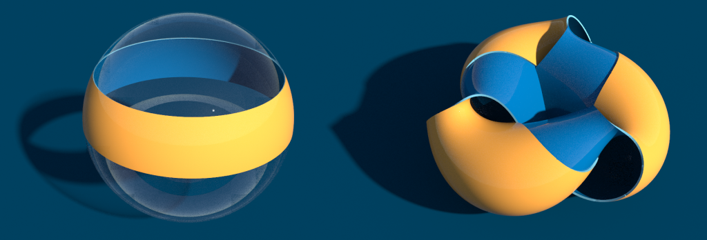
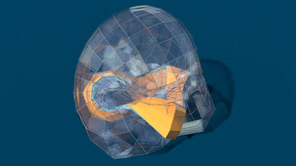
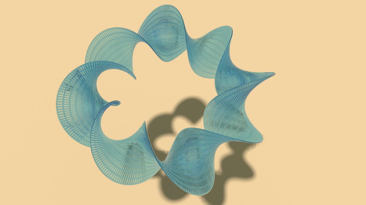
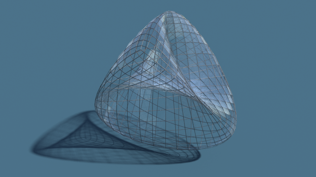
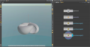
Below a quite coarse parametrization of Boy’s surface.

Homework (due 14 May): Wire up a network to visualize Boy’s surface. In detail this means:
1) Write a subnet that produces a cell decomposition of \(\mathbb R\mathrm P^2\).
2) Write a subnet that removes disks around north and south pole to obtain a strip.
3) Implement Kusner’s formula and postcompose with the sphere inversion to obtain Boy’s surface.
Build in parameters to control the resolution of the cell-decomposition, the integer \(p\) and the width of the strip.

Posted in Tutorial | Leave a comment

Smooth Dirichlet Energy and Laplace Operator

Let $M \subset \mathbb{R}^2$ be a domain with smooth boundary $\partial M$ and outpointing normal vector field $N$. For a smooth function $f \in C^{\infty}(M,\mathbb{R})$ the gradient vector field $\mbox{grad} \, f :M \rightarrow \mathbb{R}^2$ is defined as :
\[ \mbox{grad} \, f := \left( \begin{array}{c} \frac{\partial f}{\partial x} \\ \frac{\partial f}{\partial y} \end{array} \right)  = \left( f’\right)^t. \]
For a vector field $v:M \rightarrow \mathbb{R}^2$ the divergence is given by:
\[\mbox{div} \, v := \frac{\partial v_1}{\partial x} +\frac{\partial v_2}{\partial y}.\]
Taking this together we can define the laplace operator $\Delta : C^{\infty}(M,\mathbb{R})\rightarrow C^{\infty}(M,\mathbb{R})$:
\[\Delta \,f := \mbox{div} \, \mbox{grad}\, f = \frac{\partial^2 f}{\partial x^2} +\frac{\partial^2 f}{\partial y^2}.\]
The laplace operator plays an important role in physics and geometry. A typical problem from physics is the following called Dirichlet boundary problem: Given $g \in C^{\infty}(\partial M,\mathbb{R})$ find $f \in C^{\infty}(M,\mathbb{R})$ such that:
\[\left\{ \begin{array}{cc} \Delta \, f = 0 \\  \left. f\right|_{\partial M} = g.\end{array} \right.\]
If $f$ is a temperature distribution on $M$ and $g$ is the prescribed temperature on the boundary, then $f$ has to solve the heat equation: $\dot{f} = \Delta \, f.$ For a stationary temperature distribution there holds $\dot{f}=0$ and we obtain the above Dirichlet boundary problem.

Theorem:
1) Given $g \in C^{\infty}(\partial M,\mathbb{R})$ and $d \in C^{\infty}(M,\mathbb{R})$, then there is a unique $f \in C^{\infty}(M,\mathbb{R})$ such that: \[\left\{ \begin{array}{cc} \Delta \, f = d \\ \left. f\right|_{\partial M} = g.\end{array} \right.\]
2) If $d=0$ and $f$ is a solution of the corresponding Dirichlet boundary problem, then $f$ minimizes the Dirichlet energy \[ E_D(f):=\frac{1}{2}\int_M \left|\mbox{grad}\,f\right|^2,\] among all the functions $h \in C^{\infty}(M,\mathbb{R})$ with $\left. h\right|_{\partial M} = g.$

Proof:
1) The proof of the existence of $f$ is hard and can be found in some good books about PDE’s. We only proof the uniqueness of $f$.
Suppose there exists $f,\tilde{f} \in C^{\infty}(M,\mathbb{R})$ with: \( \Delta \, f =  \Delta \,\tilde{f} =0\) and \(\left. f\right|_{\partial M} =\left. \tilde{f}\right|_{\partial M} =g\), then $u:= \tilde{f} -f$ solves:
\[\left\{ \begin{array}{cc} \Delta \, u = 0 \\\left. u\right|_{\partial M} = 0.\end{array} \right.\]Now we consider the vector field $X:= u\, \mbox{grad} \,u$. For the divergence of $X$ we get:
\[ \mbox{div}\,X = \mbox{div} (u\, \mbox{grad} \,u) =\langle \mbox{grad}\,u, \mbox{grad} \,u\rangle\ + u\, \mbox{div}\, \mbox{grad} \, u =  \langle \mbox{grad}\,u, \mbox{grad} \,u\rangle\ + u \Delta \,u.\]
Using the fact that $X$ vanishes on the boundary and applying the divergence theorem we obtain:
\[0=\int_{\partial M}\langle X, N\rangle = \int_M \mbox{div}\,X = \int_M \langle \mbox{grad}\,u, \mbox{grad} \,u\rangle\ + u \Delta \,u = \int_M \left|\mbox{grad}\,u\right|^2.\]
Therefore, we have  $\mbox{grad} \,u=0$ on the whole of $M$ and $u$ is locally constant. Due to the fact that, $\left. u\right|_{\partial M} = 0$ $u$ is identically zero and therefore $f$ is unique.

2)Let $f$ be the unique solution of the Dirichlet boundary problem $\Delta \,f =0, \quad\left. f\right|_{\partial M} =g$ and $h$ an arbitrary smooth function with  $\left. h\right|_{\partial M} =g$. For $u:=h-f$ there holds $\left. u\right|_{\partial M} =0$ and we get:
\[\int_M \left|\mbox{grad},h\right|^2=\int_M \left|\mbox{grad}\,f+u\right|^2=\int_M \left|\mbox{grad}\,f\right|^2+ 2 \int_M \langle \mbox{grad}\,f ,\mbox{grad}\,u \rangle + \int_M \left|\mbox{grad}\,u\right|^2.\]
Using the usual product rule:
\[\mbox{div}(u\,\mbox{grad}\,f ) = \langle \mbox{grad}\,f ,\mbox{grad}\,u \rangle + u\, \Delta\,f, \] and the divergence theorem we obtain:
\begin{align*}2E_D(h)=\int_M \left|\mbox{grad}\,h\right|^2 &=\int_M \left|\mbox{grad}\,f\right|^2+ 2 \int_M \mbox{div}(u\,\mbox{grad}\,f ) -u\, \underbrace{\Delta\,f}_{=0}  + \int_M \underbrace{\left|\mbox{grad}\,u\right|^2}_{\geq 0}\\ &\geq \int_M \left|\mbox{grad}\,f\right|^2 + \int_{\partial M} \underbrace{u\langle \mbox{grad}\, f,N \rangle}_{=0}\\ &= \int_M \left|\mbox{grad}\,f\right|^2 = 2E_D(f).\end{align*}

$\square$

Let us now consider the space of smooth functions on $M$ that vanish at the boundary: \[V:= \left\{f \in  C^{\infty}(M,\mathbb{R}) \, \big\vert \, \left. f\right|_{\partial M}=0 \right\}\]
We can equip  $V$ with two  scalar products $\langle\!\langle \cdot, \cdot \rangle\!\rangle , \, \langle\!\langle\cdot, \cdot \rangle\!\rangle_D :V\times V \rightarrow \mathbb{R},$
\begin{align*}\langle\!\langle f, g\rangle\!\rangle &:=\int_M fg, \\ \langle\!\langle f, g\rangle\!\rangle_D & := \int_M \langle \mbox{grad}\,f ,\mbox{grad}\,g \rangle.\end{align*}
To see that $\langle\!\langle\cdot, \cdot \rangle\!\rangle_D$  is really a scalar product on $V$ one has to check that it is positive definite (symmetry and bi-linearity are obvious).
\begin{align*} & 0=\langle\!\langle f, f\rangle\!\rangle_D  = \int_M \left|\mbox{grad}\,f\right|^2 \\  \Leftrightarrow & \quad \left|\mbox{grad}\,f\right| = 0  \end{align*}
Therefore, $f$ is locally constant. With $\left. f\right|_{\partial M}=0$ one has $f=0$.

Propositon: On V the laplace operator is self adjoint, i.e. $\langle\!\langle \Delta \,f, g\rangle\!\rangle = \langle\!\langle f, \Delta \, g\rangle\!\rangle$ and  there holds: \[\langle\!\langle \Delta \,f, g\rangle\!\rangle =-\langle\!\langle f, g\rangle\!\rangle_D .\]

Proof: \begin{align*} \langle\!\langle \Delta \,f, g\rangle\!\rangle & = \int_M g\, \mbox{div} \, \mbox{grad}\, f  = \int_M  \mbox{div} (g \, \mbox{grad}\, f ) \,- \langle \mbox{grad} \,f ,\mbox{grad} \,g \rangle \\ & = \underbrace{\int_{\partial M} f \langle \mbox{grad} \,g , N \rangle}_{=0}  – \int_M \langle \mbox{grad} \,f ,\mbox{grad}\,g \rangle  \\ &=\,-  \langle\!\langle f, g\rangle\!\rangle_D \\ &= \,- \langle\!\langle g, f\rangle\!\rangle_D \\ & \,\, \vdots \\& =\langle\!\langle f, \Delta \, g\rangle\!\rangle.\end{align*}

$\square$

Posted in Lecture | Leave a comment

Differential Forms

Let $M\subset \mathbb{R}^n$ be an open set and $f:M\to \mathbb{R}^k$ a smooth map. Then for each $p\in M$ the Jacobian $f'(p)$ is a $k\times n$ matrix. The derivative $d_pf$ of $f$ at $p$ then is the linear map given by matrix multiplication with $f'(p)$:

\begin{align*}d_pf:\mathbb{R}^n &\to \mathbb{R}^k \\\\ d_pf(X)&=f'(p)X.\end{align*}

For example, if $f$ describes a regular surface in $\mathbb{R}^3$ (so $n=2$ and $k=3$), the derivative $df$ assigns to each point $p\in M$ a linear map $d_pf:\mathbb{R}^2 \to \mathbb{R}^3$ and $f'(p)$ is a $3\times 2$ matrix:

$$f'(u,v)=\left(\begin{array}{cc}|&|\\ f_u&f_v\\ |&|\end{array}\right).$$

The image of $d_pf$ is a two-dimensional subspace of $\mathbb{R}^3$ and is called the tangent plane of $f$ at $p$.

Suppose now $k=1$. Then $\omega:=df$ is a so-called 1-form on $M$, which means that $\omega$ assigns to each $p\in M$ a linear form $\omega_p:\mathbb{R}^n\to\mathbb{R}$. Let us define for $j\in \{1,\ldots,n\}$ the $j$th coordinate function $x_j:M\to \mathbb{R}$ by

$$x_j(u_1,\ldots,u_n)=u_j.$$

Then for $p=(u_1\ldots,u_n)$ and

$$Y=\left(\begin{array}{c}y_1\\ \vdots \\y_n\end{array}\right).$$

we have

$$d_px_j(Y)= y_j.$$

Each 1-form $\omega$ on $M$ can be uniquely written as

$$\omega=a_1 \,dx_1 + \ldots + a_n \,dx_n.$$

with functions $a_1,\ldots a_n:M\to \mathbb{R}$ (they always will be assumed to be smooth). For example, if $f:M\to \mathbb{R}$ is a function then

$$df=\frac{\partial f}{\partial x_1} dx_1 +\ldots \frac{\partial f}{\partial x_n} dx_n.$$

A 2-form $\sigma$ on $M$ assigns to each $p\in M$ a skew-symmetric bilinear map

\begin{align*}\sigma_p:\mathbb{R}^n\times \mathbb{R}^n &\to \mathbb{R} \\\\ \sigma_p(X,Y)&=-\sigma_p(Y,X)\end{align*}

For two 1-forms $\omega$ and $\eta$ we define a 2-form $\omega \wedge \eta$ as

$$\omega \wedge \eta (X,Y)=\omega(X)\eta(Y)-\omega(Y)\eta(X).$$

For a 1-form $\omega$ given as above by functions $a_1,\ldots a_n$ we define the exterior derivative $d\omega$ as the 2-form

$$d\omega= da_1\wedge dx_1 +\ldots +da_n \wedge dx_n.$$

For example, for $n=2$ and $\omega=a\,du + b \,dv$ we have

$$d\omega= \left(\frac{\partial a}{\partial v}-\frac{\partial b}{\partial u}\right)du\wedge dv.$$

It is clear how to multiply a 1-form or a 2-form (from the left or from the right) by a function $f:M\to \mathbb{R}$. From these definitions we derive the following rules:

\begin{align*}\omega \wedge \eta&=-\eta \wedge \omega \\\\ d(f\omega)&=df\wedge \omega+f\,d\omega \\\\ d(\omega f)&=d\omega-\omega\wedge df.\end{align*}

If $\omega$ is a 1-form on $M$ and $\gamma:[a,b]\to \mathbb{R}^n$ is asmooth curve we define

$$\int_\gamma \omega := \int_a^b \omega(\gamma'(t))dt.$$

After defining $n$-forms we could give an $n$-dimensional version of the following definition, but for now let $M$ be a compact planar domain with smooth boundary $\partial M$ and let $\sigma=\rho\, du\wedge dv$ be a 2-form on $M$. Then we define

$$\int_M \sigma:= \int_M \rho\,\, du\,dv.$$

Now we can state a special case of the most important theorem that concerns differential forms.

Theorem of Stokes: Let $\omega$ be a 1-form on a compact planar domain$M$ with smooth boundary. Then

$$\int_M d\omega =\int_{\partial M} \omega.$$


Posted in Lecture | Leave a comment

Tutorial 3: Lawson’s Minimal Surfaces and the Sudanese Möbius Band

In the last tutorial we constructed certain minimal surfaces in hyperbolic space. These hyperbolic helicoids were generated by a 1-parameter family of geodesics: while moving on a geodesic – the axis of the helicoid – another geodesic perpendicular to the axis was rotated with constant speed. It turns out that the very same procedure applied to the 3-sphere yields minimal surfaces, too.

Actually the geodesics in the 3-sphere are great circles, i.e. the intersections of the sphere with a 2-plane. Thus we end up with a family of circles. In particular the topology of the resulting surfaces will be different than in the Euclidean or the hyperbolic case. Depending on the rotation speed, we end up in basically 3 situations: 

sketch-cylinder-torus-klein

We get

  1. a cylinder: the speed is such that we never end up with the same circle going round the axis,
  2. a torus: after we traveled around the axis finitely often we end up up with the circle we started with and the surface closes up to an orientable surface, or
  3. a Klein bottle: here the surface also closes up, but the resulting surface is non-orientable.

What is a Klein bottle? Maybe we first look at a quite famous example of a non-orientable surface – the Möbius strip.

moebiusstrip_

It is the surface obtained by gluing a rectangular strip together along two opposite sides but with a twist of 180 degree. 

If the surface is smooth one possible description of non-orientability is that the surface has no non-vanishing normal vector field. Thus one cannot distinguish the sides of the surface. So to speak non-orientable surfaces have only one side. This can be easily played through on the Möbius strip – walking once around a non-contractible loop one comes back upside down.

The Klein bottle is then obtained by gluing in addition the other two sides of the rectangle. Here a schematic picture of the Möbius band (left) and the Klein bottle (right) – the arrows indicate how to glue.

moebius

On the other hand a Klein bottle can be cut it into two Möbius strips. The picture below indicates how this can be done.

kleinto2moebius

It is known that the stereographic projection of a minimal surface in \(\mathrm S^3\) is a Willmore surface. This we will use later to obtain a particularly nice Möbius strip from such a minimal Klein bottle.

So let us start with the construction of our minimal surfaces. First, like in hyperbolic space we can normalize the axis to be \(t\mapsto \gamma(t)=(\cos t,\sin t,0,0)\) – any great circle can be mapped to this curve by an isometry of \(\mathrm S^3\) (basically a rotation in \(\mathbb R^4\)). A unit length normal vector field to the axis is then certainly of the form \(t\mapsto (0,0,\cos g(t),\sin g(t))\), where \(g\) is some real-valued function. Since \(\Vert\gamma^\prime\Vert = 1\) we move along the axis with constant unit speed. Thus, up to isometry, a normal vector field \(N\) which rotates with constant speed \(\tau\in \mathbb R\) is given by \(N(t)=(0,0,\cos(\tau t),\sin(\tau t))\). The axis \(\gamma\) and the normal vector field \(N\) then let to the following easy formula for the immersion:\[f_\tau(x,y):= \cos y\, \gamma(x) + \sin y\, N(x) = \bigr(\cos y \cos x, \cos y \sin x, \sin y \cos (\tau x),\sin y \sin(\tau x)\bigr).\]

From the formula we can directly read of when this closes up – namely if and only if \(\tau = \frac{m}{n}\in \mathbb Q\). Actually these surfaces were studied by Lawson. A list of properties is given in Theorem 3 (page 351) in Lawson’s article ‘Complete minimal surfaces in \(\mathrm S^3\)’.

Given the formula, the surfaces are easy to implement. The last thing we have to do is to project it from \(\mathrm S^3\) into \(\mathbb R^3\). As we know this can be done by stereographic projection, usually from the north pole:\[\sigma\colon \mathrm S^3 \setminus \{(0,0,0,1)\} \to \mathbb R^3,\quad (x,y,z,w) \mapsto\Bigl(\frac{x}{1-w},\frac{y}{1-w},\frac{z}{1-w}\Bigr).\]Thus, at least as long as the surface does not go through the north pole, we can project the surface into Euclidean 3-space. Unfortunately, the surfaces pass through the north pole by construction. A screenshot of the result below.

screenshot

Though this is easily fixed by choosing another point to project from or, alternatively, by applying a suitable rotation to \(\mathrm S^3\) before we project it by the stereographic projection \(\sigma\). E.g. if we multiply the sphere first with \(q = (1 + \mathbf i+ \mathbf j + \mathbf k)/2\),  we find that the surface in fact looks quite nice – it is the Clifford torus (here \(\tau = 1\)).

clifford

For general \(\tau\) we get self-intersections and the surface hides what is going on ‘inside’. Below a picture for \(\tau=2\).

tau2full

Again it is helpful to restrict the domain of definition of \(f_\tau\) and render just a part of the surface. Below we restricted \(f_\tau\) to the domain \([0,2\pi]\times[-\pi/4,\pi/4]\). Here the result for the surface above.

tau2half

If we instead use \(\tau = 1/2\) we get a Möbius strip.

sudanesehalf

Extending the domain to \([0,2\pi]\times[-\pi/2,\pi/2]\) then yields a particularly nice Möbius strip – the so called Sudanese Möbius band – which is shown in the picture below. It is an embedded Willmore surface whose boundary curve is actually a round circle.

sudanese

Homework (due 7 May): Write a network that visualizes the surfaces \(f_\tau\) in \(\mathbb R^3\). Build in parameters to  change the resolution, the domain and the rotation speed \(\tau\). Finally render your own Sudanese surface.

Posted in Tutorial | Leave a comment

Quaternions

Quaternions, $\mathbb{H}$ are a number system like real or complex numbers but with 4 dimensions. In particular, $\mathbb{H}$ is nothing but $\mathbb{R}^4$ together with a multiplication law. The identification of $\mathbb{H}$ and $\mathbb{R}^4$ is given by:
$$ \mathbb{H} = \lbrace x_0 + x_1 {\bf i} + x_2 {\bf j} + x_3 {\bf k} \,\vert \,x_0,x_1,x_2,x_3 \in \mathbb{R} \rbrace.$$
With the usual addition and scalar multiplication inherited from $\mathbb{R}^4$, $\mathbb{H}$ becomes a four dimensional  $\mathbb{R}$ vector space with canonical basis $\{ 1, {\bf i}, {\bf j}, {\bf k} \}.$ The quaternion multiplication is defined by:
\begin{align*}
&\left(x_0 + x_1 {\bf i} + x_2{\bf j} + x_3 {\bf k} \right) \cdot \left(y_0 + y_1{\bf i} + y_2{\bf j} + y_3  {\bf k} \right) \\:= & \left(x_0 y_0 – x_1 y_1 – x_2 y_2 – x_3 y_3 \right) \\
+ & \left(x_0 y_1 + x_1 y_0 + x_2 y_3 – x_3 y_2 \right){\bf i} \\
+ & \left(x_0 y_2 – x_1 y_3 + x_2 y_0 + x_3 y_1 \right){\bf j} \\
+ & \left(x_0 y_3 + x_1 y_2 – x_2 y_1 + x_3 y_0 \right) {\bf k}.
\end{align*}

A more simple way to define the quaternion multiplication is to say that the multiplication with $\alpha \in \mathbb{R}$ works as usually and that ${\bf i}, {\bf j}, {\bf k}$ satisfy the following  multiplication rules:

\[{\bf i}^2 = {\bf j}^2 = {\bf k}^2 = -1,\quad {\bf ij}=-{\bf ji}={\bf k}, \quad {\bf jk}=-{\bf kj}={\bf i}, \quad {\bf ki}=-{\bf ik}={\bf j}.\]

${\rm Re}(\mathbb{H}) := span\{1\}$ is called the real part of  $\mathbb{H}$ and ${\rm Im}(\mathbb{H}) := span\{{\bf i}, {\bf j}, {\bf k}\}$  the imaginary part and there holds:  $\mathbb{H} = {\rm Re}(\mathbb{H}) \oplus {\rm Im}(\mathbb{H})$. If we identify ${\rm Re}(\mathbb{H})$ with $\mathbb{R}$ and ${\rm Im}(\mathbb{H})$ with $\mathbb{R}^3$, we can write any ${\bf x} \in \mathbb{H} $ as: $\quad {\bf x} = \alpha + {\bf v},\quad $ for some  $\alpha \in \mathbb{R}$ and ${\bf v}\in \mathbb{R}^3.$ This notation gives us a new expression of the quaternion multiplication using the scalar and cross product of $\mathbb{R}^3$:
$${\bf p}{\bf q} = (\alpha + {\bf v}) (\beta + {\bf w}) = \alpha \beta -\langle {\bf v},{\bf w}\rangle + \alpha {\bf w}+ \beta {\bf v} + {\bf v} \times {\bf w}.$$

Due to the fact that the cross product is skew symmetric, we immediately see that the quaternion multiplication is not commutative, i.e. in general there holds ${\bf p}{\bf q} \neq {\bf q}{\bf p}$.

Proposition: The quaternion multiplication is associative i.e. for ${\bf p}, {\bf q}, {\bf r} \in \mathbb{H}$ there holds:
$$ ({\bf p}{\bf q}){\bf r}={\bf p}({\bf q}{\bf r})$$

Proof: Let \[ I :=  \left(\begin{array}{cc} 1 & 0 \\0 & 1\end{array} \right), \quad X := \left(\begin{array}{cc}{\bf i} & 0 \\ 0 & -{\bf i}\end{array}\right), \quad Y := \left(\begin{array}{cc} 0 & -1 \\ 1 & 0\end{array}\right), \quad Z := \left(\begin{array}{cc} 0 & -{\bf i} \\- {\bf i} & 0\end{array}\right). \]

Now we can define a linear map \begin{align*} F:\mathbb{H} &\rightarrow \mathbb{C}^{2\times 2} \\ x_0 + x_1 {\bf i} + x_2 {\bf j} + x_3 {\bf k} &\mapsto x_0 I + x_1 X + x_2 Y + x_3 Z \end{align*}
A straight forward calculation shows that $I,X,Y,Z$ satisfy the following product rules with respect to the matrix multiplication:
\begin{align*}  I^2=I , \quad &IX=XI=I, \quad XY=-YX = Z, \\ &IY=YI =Y , \quad YZ=-ZY=X, \\ &IZ=ZI=Z, \quad ZX=-XZ =Y.\end{align*}
Therfore, $F$ is an algebra isomorphism onto its image. Due to the fact that the matrix multiplication is associative we obtain that the quaternion multiplication is associative too.

The conjugate of an quaternion number $ {\bf x} = \alpha + {\bf v}$ is given by $ {\bf\bar{ x}} = \alpha – {\bf v}$.

Proposition: For $ {\bf p}, {\bf q} \in \mathbb{H}$ there holds : $ {\bf\overline{ pq}} = {\bf\bar{ q}}{\bf\bar{ p}}.$

Proof: \begin{align*} {\bf p}{\bf q} &= \alpha \beta -\langle {\bf v},{\bf w}\rangle + \alpha {\bf w}+ \beta {\bf v} + {\bf v} \times {\bf w} \\
\overline{ {\bf p}{\bf q}} &= \alpha \beta – \langle {\bf v},{\bf w}\rangle – \alpha {\bf w} – \beta {\bf v} + {\bf w} \times {\bf v}\\
&= {\bf \bar{q}}{\bf \bar{p}}\end{align*}

$\mathbb{H}$ also inherits the euclidean norm from $\mathbb{R}^4$: $|{\bf p}| = (\sum_{i=0}^3 p_i^2)^{\frac{1}{2}}$. Similar to the complex numbers we have $|{\bf p}|^2 = {\bf p}{\bf \bar{p}}={\bf \bar{p}}{\bf p}$. Additionally, there holds the following useful formula:

Proposition: For ${\bf p},{\bf q} \in \mathbb{H}$ there holds: $|{\bf p}{\bf q}|=|{\bf p}||{\bf q}|.$

Proof:\begin{align*} |{\bf p}{\bf q}| =(({\bf p}{\bf q}) (\overline{{\bf p}{\bf q}}))^{\frac{1}{2}} = ({\bf p}{\bf q} {\bf \bar{q}}{\bf \bar{p}})^{\frac{1}{2}}  = ({\bf p} |{\bf q}|^2{\bf \bar{p}})^{\frac{1}{2} } = (|{\bf p}|^2 |{\bf q}|^2)^{\frac{1}{2} } = |{\bf p}||{\bf q}|. \end{align*}

Note that for ${\bf q} \in \mathbb{H}$ the inverse element with respect to the quaternion multiplication is given by
$${\bf q} ^{-1} = \frac{{\bf \bar{q}} }{|{\bf q}|^2 }.$$
For quaternions with unit length this gives us immediately ${\bf q} ^{-1} = {\bf \bar{q}}.$
What makes quaternions so useful is the fact that one can describe rotation in $\mathbb{R}^3$ with them in a very elegant way. Therefore, we have to consider $\mathbb{R}^3$ as ${\rm Im}(\mathbb{H})$.

Theorem: Let ${\bf a} \in \mathbb{R}^3$ with $|{\bf a}|=1$ , $\alpha \in \mathbb{R}$ and ${\bf q} = \cos\left(\frac{\alpha}{2}\right) + \sin\left(\frac{\alpha}{2}\right) {\bf a}$. Then for all ${\bf y} \in \mathbb{R}^3$ we have:

(i)  ${\bf q}{\bf y} {\bf \bar{q}} \in {\rm Im} (\mathbb{H}) = \mathbb{R}^3$

(ii) The map $F:\mathbb{R}^3 \rightarrow \mathbb{R}^3$, ${\bf y} \mapsto {\bf q}{\bf y}{\bf \bar{q}}$ is a rotation around ${\bf a}$ by the angle $\alpha$.

Proof: (i) First note that a quaternion ${\bf y}$ is purely imaginary if and only if ${\bf \bar{y}}= -{\bf y}$. Thus we have to show $\overline{{\bf q}{\bf y}{\bf \bar{q}}}= \,- {\bf q}{\bf y}{\bf \bar{q}}$.
$$\overline{{\bf q}{\bf y}{\bf \bar{q}}} = {\bf q}{\bf \bar{y}}{\bf \bar{q}} = \,- {\bf q}{\bf y}{\bf \bar{q}}.$$

(ii) $F$ is a linear map and therefore completely determined by its action on a basis. We extend ${\bf a}$ to an positive oriented  orthonormal basis $\{{\bf a}, {\bf b}, {\bf c} \}$ of $\mathbb{R}^3$.
\begin{align*}F({\bf a}) = {\bf q}{\bf a}{\bf \bar{q}} &= \left( \cos\left(\frac{\alpha}{2}\right) + \sin\left(\frac{\alpha}{2}\right) {\bf a}\right) {\bf a}\left(\cos\left(\frac{\alpha}{2}\right) – \sin\left(\frac{\alpha}{2}\right) {\bf a}\right) \\ &= \left( \cos\left(\frac{\alpha}{2}\right) + \sin\left(\frac{\alpha}{2}\right) {\bf a}\right)\left(\cos\left(\frac{\alpha}{2}\right){\bf a} + \sin\left(\frac{\alpha}{2}\right)\right ) \\ &= \left( \cos^2\left(\frac{\alpha}{2}\right) + \sin^2\left(\frac{\alpha}{2}\right)\right) {\bf a} + \cos\left(\frac{\alpha}{2}\right) \sin\left(\frac{\alpha}{2}\right) (1+{\bf a}^2) \\ & =  {\bf a}.\end{align*}

In the last step we used that ${\bf a}^2= \,-1$. This gives us that  the ${\bf a}$-axis is invariant under $F$. Now we consider the action of $F$ on the plane orthogonal to ${\bf a}$, i.e. the plane spanned by $ {\bf b}$ and ${\bf c}$. Since $ \langle {\bf a}, {\bf b} \rangle =0 $ we have:
$$ {\bf a}{\bf b} = {\bf a} \times {\bf b} = \,- {\bf b} \times {\bf a} = \,- {\bf b}{\bf a}.$$

Using this and the addition formulas for cosine and sine we get:
\begin{align*} F({\bf b}) & = \left( \cos\left(\frac{\alpha}{2}\right) + \sin\left(\frac{\alpha}{2}\right) {\bf a}\right) {\bf b} \left(\cos\left(\frac{\alpha}{2}\right) – \sin\left(\frac{\alpha}{2}\right) {\bf a}\right) \\ &= \left( \cos\left(\frac{\alpha}{2}\right) + \sin\left(\frac{\alpha}{2}\right) {\bf a}\right) \left(\cos\left(\frac{\alpha}{2}\right) + \sin\left(\frac{\alpha}{2}\right) {\bf a}\right)  {\bf b} \\ &=\left( \cos(\alpha) + \sin(\alpha) {\bf a}\right) {\bf b} = \cos(\alpha){\bf b} + \sin(\alpha)\left( {\bf a} \times {\bf b}\right) \\ &=  \cos(\alpha){\bf b} + \sin(\alpha) {\bf c}\end{align*}

Analog we obtain $F({\bf c}) =  \cos(\alpha){\bf b} – \sin(\alpha) {\bf b} $ and the matrix representation of $F$ with respect to the basis  $\{{\bf a}, {\bf b}, {\bf c} \}$ is given by:
\[ F =  \left(\begin{array}{ccc} 1 & 0 & 0 \\0 & \cos(\alpha) & -\sin(\alpha) \\ 0 & \sin(\alpha) & \cos(\alpha) \end{array} \right)\].

Now it is easy to see that $F$ describes a rotation around ${\bf a}$ by the angle $\alpha$.

Corollary: For every $ {\bf q} \in \mathbb{H}\backslash \{0\}$ the map $F:\mathbb{R}^3 \rightarrow \mathbb{R}^3$, ${\bf y} \mapsto {\bf q}{\bf y}{\bf q}^{-1}$ is a rotation.

Proof: With ${\bf q} ^{-1} = \frac{{\bf \bar{q}} }{|{\bf q}|^2 }$ we get:
$$ {\bf q}{\bf y}{\bf q}^{-1} = \frac{{\bf q}}{|{\bf q}|}{\bf y}\overline{\left(\frac{{\bf q} }{|{\bf q}| }\right)}$$
Since $\frac{{\bf q}}{|{\bf q}|}$ has unit length there exists ${\bf a} \in \mathbb{R}^3$ with $|{\bf a}|=1$ and  $\alpha \in \mathbb{R}$  such that: $\frac{{\bf q}}{|{\bf q}|} = \cos\left(\frac{\alpha}{2}\right) + \sin\left(\frac{\alpha}{2}\right) {\bf a} $ and we can apply the theorem.

Note that the quaternion multiplication corresponds to the concatenation of rotations. Let ${\bf p}, {\bf q} \in \mathbb{H}$ with $|{\bf p}|= |{\bf q}| =1$ and $F,G:\mathbb{R}^3 \rightarrow \mathbb{R}^3$ the corresponding rotations i.e. $F({\bf y}) = {\bf q}{\bf y}{\bf \bar{q}}$ and $G({\bf y}) = {\bf p}{\bf y}{\bf \bar{p}}$, then we get for the concatenation:

$$\left( F \circ G\right) (y) = {\bf q}\left( {\bf p}{\bf y}{\bf \bar{p}} \right) {\bf \bar{q}} = \left({\bf q} {\bf p}\right){\bf y}\overline{\left({\bf q} {\bf p}\right)}.$$

Posted in Lecture | Leave a comment

Tutorial 2: Hyperbolic Helicoids

A ruled surface is a surface in \(\mathbb R^3\) that arises from a 1-parameter family of straight lines, i.e. these surfaces are obtained by moving a straight line though the Euclidean space. E.g. a normal vector field of a curve defines such a rule surface:

ruledsurface_

The plane is a ruled surface which – like a soap film – locally minimizes the area, a so called minimal surfaceAnother, more interesting, ruled minimal surface is the catenoid. Not counting the plane it was the first minimal surface which was discovered and it turns out that with the plane it is the the only rotationally symmetric minimal surface.

associatefamily

Like all minimal surfaces the catenoid comes with a whole 1-parameter family of minimal surfaces – the so called associate family – also containing the helicoid which arises as the skew motion of a straight line along a fixed perpendicular straight line.

The whole family has a closed form expression: For each \(\alpha\in(-\pi,\pi]\) a conformal parametrization is given by\[f\colon (-\pi,\pi]\times\mathbb R \to \mathbb R^3, \quad (x,y) \mapsto \begin{pmatrix}\cos\alpha\,\sinh y\, \sin x + \sin\alpha\, \cosh y\, \cos x \\ -\cos\alpha\,\sinh y\, \cos x + \sin\alpha\, \cosh y\, \sin x \\ x\,\cos \alpha + y\sin\alpha\end{pmatrix}.\]

Exercise: Build a network that visualizes the associated family of the catenoid.

The helicoid construction provides minimal surfaces in hyperbolic 3-space In this tutorial these hyperbolic helicoids shall be visualized.

We start with the Poincaré half space model of the hyperbolic 3-space: Here the hyperbolic space is represented by the upper half plane \(\mathrm H^3 = \{(x,y,z)\in\mathbb R^3\mid z>0\}\). Though the angles stay the same, distances in \(\mathrm H^3\) are measured differently from the Euclidean half space.

With this notion of distance the hyperplane \(\mathrm E=\{(x,y,z)\in\mathbb R^3\mid z = 0\}\) has infinite distance to each point of \(\mathrm H^3\) and the shortest path between two points is realized by arcs of circles perpendicular to \(\mathrm E\):

geodesicshalfspacemodel

Such locally shortest paths are called geodesics and are the equivalent of straight lines in non-Euclidean geometry. In Euclidean space a helicoid is a straight line, i.e. a geodesic, which rotates with a constant speed while moving on another perpendicular straight line. So in analogy to Euclidean case the hyperbolic helicoids appear by rotating a geodesic (circle perpendicular to \(\mathrm E\)) with constant speed while moving along another geodesic.

This might sound complicated first. Though, the isometries of hyperbolic space turn out to be exactly the Möbius transformations preserving the hyperplane \(\mathrm E\) and any two geodesics can be mapped onto each other by such a Möbius transformation. This allows us to fix the geodesic we move along to be the \(z\)-axis and drastically simplifies the setup: The distance between two points \(p,q\in\mathrm H^3\) that lie on the \(z\)-axis is given just as follows\[d(p,q) = |\ln b\, -\, \ln a\,|,\quad p=(0,0,a),\,q=(0,0,b).\]With this we can construct all hyperbolic helicoids as follows: Let \(\tau\in \mathbb R\) and \(\mathbf v \in \mathrm E\) be of unit length with respect to the standard product of \(\mathbb R^3\), then a parametrization of the hyperbolic helicoid is given by\[f\colon \mathbb R\times(-\tfrac{\pi}{2},\tfrac{\pi}{2}) \to \mathbb R^3,\quad (x,y) \mapsto \cos y\, \Bigl(\begin{smallmatrix}0\\0\\e^x\end{smallmatrix}\Bigr) +\sin y\,e^x\,\Bigl(\cos(\tau x)\,\mathbf v + \sin(\tau x)\,e_3\times \mathbf v\Bigr).\]Here, as usual, \(e_3\) denotes the third basis vector of the standard basis of \(\mathbb R^3\): \(e_3 = (0,0,1)\). All other hyperbolic helicoids are obtained then by postcomposition with Möbius transformations that leave \(\mathrm E\) invariant.

hyperbolichelicoid_

For this particular rendering we equipped the ground with the default clay material and changed its color to a deep blue. The helicoid itself was thickened by a polyextrude node and equipped with whiteporcelain material the color of which we changed to orange. For the light we used the arealight.

Most of the geometry is hidden in this view. Thus it might be better restrict the map \(f\) to \([-\alpha,\alpha]\times \mathbb R\) for \(0<\alpha<\pi\). This amounts to restricting the image to a cone.

hyperbolichelicoidcone_

An even better visualization can be achieved by mapping the upper half-plane by a Möbius transformation to unit ball. This map can be achieved by a combining translations and an inversion \(T\) in the unit sphere: First we shift the half space up by adding \(e_3\). If we then apply \(T\) it is mapped to a sphere of radius \(\tfrac{1}{2}\) with center \((0,0,\tfrac{1}{2})\).

sphereinversion

Rescaling by \(2\) and subtracting \(e_3\) yields then a Möbius transformation that sends the upper half plane to the ball of radius \(1\). Altogether the map is given by\[x\mapsto 2\frac{x+e_3\,}{\Vert x+e_3\Vert^2}-e_3.\]Actually by this transformation we get another model of the hyperbolic space known a the Poincaré disk model.

The ball itself can be nicely incorporated in the picture by drawing a unit sphere, which is equipped with the glass material.

hyperbolichelicoidball_

Since Möbius transformations are conformal the angles are preserved under this transformation. Further circles (or straight line) are mapped to circles (or straight lines). Thus the straight lines in the cone are mapped to circles all passing through to points on the boundary of the disk – the images of \(0\) and \(\infty\) under the Möbius transformation. Thus the helicoid is bounded by a spindle like surface.

imageofcone

hyperbolichelicoidconeball_

Homework (due 30 April): Visualize the hyperbolic helicoids, i.e. implement the construction described above which yields a helicoid that connects the south to the north pole. Use a Möbius transformation to obtain a helicoid that connects the south pole with an arbitrary given point on the 2-sphere.

hyperbolichelicoidballbent_

Posted in Tutorial | Leave a comment

Tutorial 1: Möbius Transformations

In this first tutorial we build a simple network to visualize Möbius transformations of a given geometry—below a picture of a cube together with its Möbius transform.

The Möbius transformations are the group of transformations of \(\mathbb R^n\cup\{\infty\} \cong \mathbb S^n\) generated by the Euclidean transformations (rotations + translation) together with inflections in spheres: The inflection in the sphere of radius \(r>0\) with center \(m=0\) is given by\[x\mapsto r^2 \frac{x}{|x|^2}\,.\]In particular, the group contains scalings. Though these maps distort the lengths, they still preserve angles.

While there are a lot of angle preserving maps mapping \(\mathbb R^2\) to itself (holomorphic maps away from critical points), Liouville’s theorem tells us that in dimension \(n>2\) conformal transformations are Möbius transformations.

On the picture above one can get the impression that the side and edges of the cube are bent to spherical squares and circle arcs. In fact, this is true: Möbius transformations map generalized spheres to generalized spheres.  Where a generalized sphere refers to a spheres or a plane—a sphere of infinite radius.

To get a feeling what an inflection in a sphere does, we set up a simple network. We start with an embedded cube \(f\colon \mathbb S^2 \to \mathbb R^3\) and post-compose it with an inflection in a given sphere\(g\) to obtain a new embedding\[\tilde f = g\circ f\,.\]

In Houdini this means we generate a cube, e.g. using a box node (make sure that its parameter primitive type is set to ‘polygon mesh’), and modify then its point positions (the point attribute v@P) by a Möbius transformation using a point wrangle node.

To see both the original cube and the transformed cube we can use a merge node, which merges the two geometries in just one. The VEX code in point wrangle node which does the inversion in the unit sphere is very minimalistic. It just contains one line:

v@P /= length2(v@P);

If you now drag around the original cube you can see how the transformed cube changes. Though the transformed cube still has planar faces and not—as it should have—spherical ones. This is due to the coarse resolution. To obtain a better approximation we need to subdivide the original cube—this can be done directly by setting parameters (‘axis divisions’) of the box node.

Let us decorate the edges and vertices of the (not subdivided) cube. Therefore we use a wireframe node to paint tubes around its edges and a copy to points node to put spheres to its 8 vertices.

To have both a cube and a subdivided and we set a second box node with center and scale copied from the box1. This can be done by writing ch("../box1/scale") into the Uniform Scale parameter of the second box node box2. Similarly with the center parameter.

Similarly we can decorate the transformed cube . Only here we need to subdivide the edges so to see that they form circle arcs—this can be done by wiring a resample node as shown below.

The nodes pointwrangle2 and pointwrangle3 in the network are just copies of pointwrangle1. Here is how the result should look like.

For the inflection we just used the unit sphere. Certainly, it is good to have the sphere also visible in the scene. Therefore we just place a sphere node and merge its geometry to the cube geometries. If one chooses the sphere to be a mesh one can set the f@Alpha point attribute (responsible for opacity) to e.g. 0.1 so that we have a transparent sphere. This is done again by a point wrangle node.

Moreover, given a sphere as explicit draggable geometry we want to make the inflection dependent on this geometry. To do this we access the parameters of the sphere node inside the point wrangle node that performs the Möbius transformation by the VEX function chf (see also this post;).

float r = chf("../sphere3/scale");
float tx = chf("../sphere3/tx");
float ty = chf("../sphere3/ty");
float tz = chf("../sphere3/tz");

In general, Möbius transformations can lead to large length distortion—the whole geometry can sometimes ‘swap over infinity’.

Thus it sometimes might be more convenient to use two sphere inflections instead. So one can easily make a setup such that the cube is contained in one and its transform is contained in the other sphere, as show in the teaser image.

Homework (due 23 April): Build up a network that visualizes the a cube and its inversion in a given sphere, as described above. In particular, make the transform dependent on the center and the radius of the sphere.

Posted in Tutorial | Leave a comment