At a student seminar at the TU Berlin in fall 2013, the following problem in plane geometry  was posed, “Given a point lying on a line, and a second point lying on a second line, find the unique direct isometry mapping the first point/line pair to the second.”  The original context was the hyperbolic plane, in thinking about the problem I realized I could solve it in a metric-neutral way, and this blog post and its sequels present that solution. I chose the title since the solution is based on an nifty tool called projective geometric algebra (PGA), and I can’t think of a better introduction to PGA than working out a concrete example like this one.  Buckle your seat belts and enjoy the ride!

What I want to do in this post:

1. Demonstrate an interactive application for playing with this problem.
2. Derive a solution for the problem in the euclidean plane.
3. Discuss some exceptional configurations and show how they can be handled within the context of the projective model of euclidean geometry in a seamless fashion.
4. Indicate how the approach leads to a “cool tool”: projective geometric algebra, a subject for a future post.

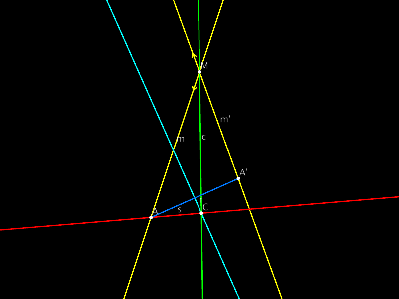
I’ve also implemented this result in a jReality webstart application.  If you start this application up, you should see a picture like the following:

Directions for using the webstart. To begin with, you may need to display the control panel to the left of the graphics window. To do this, select the menu item “Window->Left slot” (and deselect “Window->right slot” if you wish).  This is necessary due to a heightened security in Java 7 which prevents correct reading of the built-in property file (which should set these window slots properly.)

If you’re using the webstart application, you can drag any of the three points $\mathbf{A}$, $\mathbf{A’}$ and $\mathbf{M}$ and the diagram adjusts accordingly.  Use the slider labeled time to see how the rotation acts, also to confirm that the rotation actually does what is claimed. Furthermore, to reverse the orientation of either line $\mathbf{m}$ or $\mathbf{m’}$, click on the line; the orientation arrow on the line should flip and the angle bisector $\mathbf{c}$ switches accordingly to the supplementary angle.  Finally, you can switch the metric used using the combo box on the left inspector panel to choose the hyperbolic or elliptic metric also.  The given data remains the same, but the construction is carried out using this metric instead of the euclidean one.  This “metric neutral” capability will be more fully discussed in a later blog.

Return to the geometric problem. Here we want to focus on the challenge of finding a euclidean isometry which moves the point $\mathbf{A}$ to the point $\mathbf{A’}$, and the line $\mathbf{m}$ to the line $\mathbf{m’}$.  (The two lines should be thought of as oriented, so that the orientation is preserved by the isometry.) We claim that the solution is a rotation around point $\mathbf{C}$,  the intersection of line  $\mathbf{r}$ (cyan) and line $\mathbf{c}$ (green). $\mathbf{r}$ is the perpendicular bisector of the segment $\mathbf{AA’}$, while $\mathbf{c}$ is the angle bisector of the angle formed by $\mathbf{m}$ and $\mathbf{m’}$.

Indeed, the center $\mathbf{C}$ of a rotation moving $\mathbf{A}$ to  $\mathbf{A’}$ must lie the same distance to both points, which is the defining condition of $\mathbf{r}$.  Similarly, since the desired rotation maps $\mathbf{m}$ to $\mathbf{m’}$,  the closest point of $\mathbf{m}$ to $\mathbf{C}$ is mapped to the closest point of $\mathbf{m’}$ to $\mathbf{C}$, hence $\mathbf{C}$ lies the same distance to both points.  This condition is satisfied exactly by points on the angle bisector $\mathbf{c}$ of the two lines. (Here one must be careful to specify which angle bisector one means. This depends on the relative orientation of the two lines, and is easy to determine.) Hence the center of the desired rotation must lie on $\mathbf{r}$ and on $\mathbf{c}$, so it is the intersection of these two lines, as shown in the diagram.

Once the center has been found, it´s not hard to express the desired rotation as the composition of two reflections in lines passing through $\mathbf{C}$: first in the line $\mathbf{s}$ (red) followed by reflection in line $\mathbf{r}$ (cyan).  Why does this produce the desired rotation? Clearly reflection in $\mathbf{s}$ fixes $\mathbf{A}$ while that in $\mathbf{c}$ maps $\mathbf{A}$ to $\mathbf{A’}$.  Since $\mathbf{C}$ is fixed by the composition, it must be the rotation we are looking for.  Writing the reflection in line $\mathbf{s}$ as $\mathbf{R_s}$, the rotation is then the composition $\mathbf{R_C} := \mathbf{R_c}\circ \mathbf{R_s}$.

Exceptional configurations. It’s interesting to review the construction for possible exceptional configurations.  For example, $\mathbf{m}$ and $\mathbf{m’}$ may be parallel; then their intersection $\mathbf{M}$ is a so-called point at infinity or, more neutrally,  ideal point.  What is the angle bisector $\mathbf{c}$ in this case?  If the two lines have different orientations (that is, translate one to the other and compare the orientations), then the angle bisector $\mathbf{c}$ is the mid-line, parallel to both, and the construction continues as before.  If not, then $\mathbf{c}$ is the line at infinity itself (!), and the construction continues as before.

Or, $\mathbf{c}$ and $\mathbf{r}$ may be parallel; then their intersection $\mathbf{C}$ is a so-called point at infinity or ideal point, and $\mathbf{s}$, since it goes through $\mathbf{C}$ too, is also parallel to these lines.  Hence the product of the two reflections is not a rotation but a translation.  A bit poetically, one can say, a euclidean translation is a rotation around a point at infinity — by a vanishing angle!

A further exceptional configuration can occur if the lines $\mathbf{r}$ and $\mathbf{c}$ are the same line.  Then they don’t have a well-defined intersection.  It’s not hard to see that this can happen only when $\mathbf{A}$ and $\mathbf{A’}$ lie the same distance from $\mathbf{M}$, so I can rotate $\mathbf{A}$ into $\mathbf{A’}$ by a rotation around $\mathbf{M}$.  Now, if the  orientations of $\mathbf{m}$ and $\mathbf{m’}$ are preserved when I perform this rotation, then it is the desired rotation, and I can construct it by setting $\mathbf{C}$ to $\mathbf{M}$ and continuing as before; if not, the desired rotation center is found by constructing the perpendicular line $\mathbf{a}$ to $\mathbf{m}$ at $\mathbf{A}$; then the intersection of $\mathbf{a}$ and $\mathbf{c}$ is the desired rotation center $\mathbf{C}$ and the construction can continue as before.

Are there other exceptional configurations?  Please post as comment any other ones you find!

The path to geometric algebra. The observant reader will not have missed noting that the correct solution of the exceptional configurations described above proceeded a bit magically.  In particular, finding the correct solution for the first two configurations involved the ideal points and line of the euclidean plane.  These are concepts which are not necessarily associated to euclidean geometry.  That they can be used is due to the discovery by Arthur Cayley and Felix Klein in the 1860’s that projective space can be converted into a metric space in many ways by selecting a quadratic form, the so-called Absolute of the metric space.  Details lie outside the scope of this blog, see my thesis, chapter 4. This Cayley-Klein construction can be directly applied when the quadratic form is non-degenerate, and produces most importantly elliptic (or spherical) and hyperbolic space of any dimension.  It also works for euclidean space, but requires a degenerate quadratic form (some subspaces consist of points with vanishing norm).

For this post, the relevant object is the projective model of the euclidean plane.  Then the points of vanishing norm form a line, the so-called ideal line of the euclidean plane. Parallel lines meet in points of this line. This circumstance allowed us to handle the first two exceptional configurations above, where we sought the intersection of two parallel lines. In almost every euclidean construction or proof there arise such configurations, which have to be handled separately if one is relying of “traditional” euclidean geometry, but which in the context of “projective” euclidean geometry can be handled uniformly. For this reason, the projective model of euclidean geometry has clear advantages over the traditional approach.  In order to carry this out in a rigorous fashion, its useful to translate things into in the correct algebraic setting.

The traditional way of proving that the construction outlined above is correct relies on converting the steps into expressions in vector analysis of the plane.  This approach avoids mention of ideal points and line, and is limited to the euclidean setting.  Is there a better algebraic tool for the job?  In fact, there is a much more comprehensive algebraic structure — which includes vector analysis as a small sub-algebra — such that every step of the above construction can be expressed by a single compact expression. Furthermore, even though the steps of the construction are made based on the euclidean metric, the resulting expressions also provide a correct representation of the same construction when the underlying metric is elliptic or hyperbolic. The differences that arise express naturally the differences between these metrics.  For example, in elliptic space there are no parallel lines. This “metric neutrality” is an expression of  the Cayley-Klein construction underlying this approach. The webstart application allows the user to use these other metrics and confirm that the result is, in fact, metric neutral.

The same comments made regarding the projective model of the euclidean plane apply also to the hyperbolic plane.  Instead of having just one line of ideal elements, in the hyperbolic case there are a circle’s worth of ideal points and lines, and beyond them a second model of hyperbolic geometry, the polar hyperbolic plane, described briefly above. They are not part of the traditional definition of the hyperbolic plane, but can be integrated in an effortless way into the standard model of the hyperbolic plane with the advantage that all projective elements have a significance in hyperbolic geometry, not just the points of the unit disk.  This geometry can also be integrated into the algebraic structure mentioned above.

This algebraic structure is called projective geometric algebra.  I’ll share the details of this algebraic “translation” of our construction problem here in a subsequent post on this blog.