This post builds on the previous one, but returns to the original problem of finding the axis of a hyperbolic isometry.  We show that by using the projective model of hyperbolic geometry one can directly adapt the euclidean solution to obtain the hyperbolic solution also.

The hyperbolic case. The webstart, as explained above, also includes an option to switch the metric to elliptic or hyperbolic We want now to discuss the latter option.  Then the figure includes the unit circle, the boundary of the hyperbolic plane, as the following figure shows:

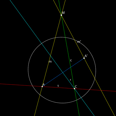
Does the description of the euclidean construction carry over to the hyperbolic case pictured above?  Clearly there are some constraints on the configuration if there is to be a solution.  For example, the points $\mathbf{A}$ and $\mathbf{A’}$ must be hyperbolic points, and the lines $\mathbf{m}$ and $\mathbf{m’}$ must also be hyperbolic.  But their intersection $\mathbf{M}$ does not need to be hyperbolic; it can be ideal (lie on the unit circle) or also hyper-ideal (lie outside).  Assuming these conditions are met, as they are in the above figure, how does the construction proceed?

The definition of the perpendicular bisector $\mathbf{r}$ is valid.  But what is the angle bisector $\mathbf{c}$ of an angle which, as in this case,  lies outside the hyperbolic disk?  As in the euclidean case, the traditional approach to hyperbolic geometry does not define this.  However, in the projective model one can define it meaningfully.  To do so, one must invoke an involutive correlation $\mathbf{\Pi}$ (a fancy name for a transformation which switches points and lines,  and whose square is the identity) on the projective plane known as the polarity on the metric quadric.  This transformation sends a point $\mathbf{P}$ to the line $\mathbf{P^\perp}$ consisting  of points whose inner product with $\mathbf{P}$ is 0, the orthogonal complement with respect to the hyperbolic metric.

The result is that one obtains a second model of the hyperbolic plane in the exterior of the unit disk, in which the roles of point and line have been reversed.  Then, for example, the point $\mathbf{M}$ when it lies outside the hyperbolic plane, is polar  to the common orthogonal line of $\mathbf{m}$ and $\mathbf{m’}$ inside the hyperbolic disk, and the angle bisector of these two lines is polar to the midpoint of this common orthogonal segment.  Proceeding in this way, one can show that the desired metric properties can be “mirrored” from the exterior of the hyperbolic plane to the interior and hence that the construction given above also solves the given problem for the hyperbolic plane too, although some of the steps may look unfamiliar, since they may involve polar entities, but the metric relations remain unchanged.  A full discussion of this phenomena lies beyond the scope of this post, but hopefully you can get a sense of how the polarity operator in effect produces two hyperbolic planes such that every metric relationship in one is mirrored (with points and lines reversed) in the other.

We leave the same positive conclusion for the elliptic plane for the never-tiring reader.  Here the situation is simplified since there are no real ideal points, every point of the projective plane is also a point of the elliptic plane and any configuration of the initial data is valid, and the construction carried out in the euclidean case goes through here without difficulties.

Having shown that the projective model of these three metric planes provides a reliable basis for solving the construction problem posed in the first post, and doing so in a metric-neutral way, the next post will provide the promised introduction to projective geometric algebra, by giving a (metric-neutral) algebraic formulation of the construction which has formed the content of this and the previous post.