In the last post I announced a contest to produce an image for the conformal map movie which is very close to being finished now. The contest didn’t attract any entries, which is understandable considering how busy a student’s life these days is.  So … I ended up producing a solution myself:

When this image is used for the texture instead of the checkerboard, the result looks like this:

Sharp-eyed readers will note that two copies of the image go together to cover the rectangle once.  Furthermore, there is a close connection between the letter ‘A’ and the new texture image.  Can you figure out what it is? Hint: make a list of the objects which appear in the image. There should be at least 11 different reasons for this connection. Can you find them all?

[Question to my readers: is there a way to get a compact enumeration in this blog?  If I write a list using the list menu item in the wordpress editor, the entries are    v e r y    f a r     a p a r t.

This post picks up where the last one left off.  Our task here is to present the essentials of projective geometric algebra and use to obtain a metric-neutral formulation of the solution to the problem discussed in the previous two posts.

Projective space to the rescue. To obtain the projective models of the metric planes of interest, begin with the  vector space $\mathbb{R^3}$ and projectivize it to produce the real projective plane $\mathbf{P}^2$.  Define an exterior algebra $\bigwedge{\mathbf{P}^2}$ by defining the points of $\mathbf{P}^2$ to be the 1-vectors.  Take the scalar field $\mathbb{R}$ as the 0-vectors.  Create the higher grades using the anti-symmetric wedge product $\wedge$.  $\mathbf{x} \wedge \mathbf{y}$ is a 2-vector,  the joining line of the arguments. The wedge of three linearly independent points $\mathbf{x} \wedge \mathbf{y} \wedge \mathbf{z}$ is the projective plane itself, and is called a pseudo-scalar.

Duality to the rescue. We can do the same with the dual algebra.  Then the 1-vectors are lines and the wedge operation is the meet of two lines. By a little bit of abstract nonsense, we can in fact restrict our attention to one of these algebras and “import” the other wedge product when we need it (by using Poincare duality, the details are in my thesis).  For our purposes we write the join operator as $\vee$ and the meet operator as $\wedge$ (note this choice is motivated to be consistent with the related set-theoretic operations union $\cup$ and intersection $\cap$). For a good intro to exterior algebras see this wikipedia article.

Adding a metric. To work in the metric relations, we have to incorporate the inner product with this outer product.  To do so we define three different signatures for our inner product: (+++), (++-), and (++0), which corresponds to elliptic, hyperbolic and euclidean plane, resp.  Write the inner product of two 1-vectors with respect to the chosen inner product as $\mathbf{m}\cdot \mathbf{n}$.  We begin with the dual exterior algebra (where 1-vectors are lines) and define a geometric product on the 1-vectors via: \[  \mathbf{m}\mathbf{n} := \mathbf{m}\cdot \mathbf{n} + \mathbf{m}\wedge \mathbf{n}\]  Note that this product is the sum of a 0-vector (a scalar) and a 2-vector. This product can be extended to all grades just by writing every k-vector as a sum of products of orthogonal basis 1-vectors (which is always possible), and reducing the products whenever the square of a basis 1-vector occurs (since the square of a 1-vector is a scalar).  In this way one obtains an associative algebra, called the Clifford or geometric algebra, characterized by its signature.  This is the projective geometric algebra we have been promising to describe.  We denote the three algebras of interest as $\mathcal{C}_\kappa$ where $\kappa$ takes on the three values of $\{-1,0,1\}$ (hyperbolic, euclidean, elliptic, resp.) To be precise, we work with an orthonormal basis for the  1-vectors $\{\mathbf{e_0}, \mathbf{e_1},\mathbf{e_2}\}$ with the metric relations given by $ \mathbf{e_0}^2 = \kappa$, $ \mathbf{e_1}^2= \mathbf{e_2}^2 = 1$.

Why (++0) is euclidean: In $\mathbb{R}^2$, consider two  lines $m_{1} : a_{1}x+b_{1}y+c_{1}=0$ and $m_{2} : a_{2}x+b_{2}y+c_{2}=0$.  Assuming WLOG $a_{i}^{2}+b_{i}^{2} = 1$, then $\cos{\alpha} = a_{1}a_{2}+b_{1}b_{2}$, where $\alpha$ is the angle between the two lines: changing the $c$ coefficient translates the line but does not change the angle it makes to other lines. That means, the $c$ coefficient makes no difference when we measure the angle between two lines.  Thus $(++0)$ is the correct choice for the inner product for euclidean planar geometry.

Why we have to use the dual algebra: If you’re wondering why we started with the dual exterior algebra, that answer is: because that’s how God make the world we live in.  Euclidean lines are less degenerate than euclidean points.  If you try to start with the standard exterior algebra (where 1-vectors are points) you cannot obtain euclidean geometry; you end up with dual euclidean geometry, in which points are less degenerate than lines, which does not at all match up with the space we live in.  (It’s a fascinating space in its own right and I hope to post something on it in the near future.)

Normalizing. It’s useful to work with normalized points and lines.  To obtain this normalization, notice that $\mathbf{m}^2$ for a 1-vector or 2-vector is a scalar. Define the norm $\|\mathbf{m}\| := \sqrt{| \mathbf{m}^2 |}$.  Then when $\| \mathbf{m} \| \neq 0$, $\dfrac{\mathbf{m}}{\| \mathbf{m}^2 \|}$ has unit norm.  For the three metric geometries we are working with, the proper points and lines always can be normalized to have square -1 and +1, resp. (In  fact, that can serve as a definition of what it means to be proper.)

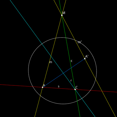
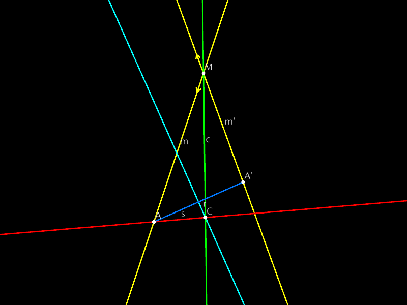
Implementing the construction. Here are the steps of the construction, translated into $\mathcal{C}_\kappa$.   The elements in the above diagram have been embedded in the natural way into the Clifford algebra as 1- or 2-vectors. We assume that all points and lines are normalized in the formulas which follow, since it simplifies the formulas.  (Normalizing ideal points is a tricky issue which we skip over in this abbreviated account.  See my thesis.)  For example, this allows us the find midpoints and angle bisectors by simply adding together the two arguments.  In the formulas below, $\mathbf{X}$ is an arbitrary point or line.  $\mathbf{R_x}$ is the geometric reflection in the line $\mathbf{x}$. $\mathbf{R_C}$ is the desired rotation around the point $\mathbf{C}$. The exceptional configurations have not been taken into account in this description.

$\begin{align} \mathbf{M} &:= \mathbf{m} \wedge \mathbf{m’} &&\text{Intersection of the two lines}  \\ \mathbf{a} &:= \mathbf{A} \vee \mathbf{A’} &&\text{joining line of the two points} \\ \mathbf{A_m} &:= \mathbf{A} + \mathbf{A’} && \text{midpoint of the two points} \\ \mathbf{r} &:= \mathbf{A_m} \mathbf{a} &&\text{perpendicular bisector of AA’} \\ \mathbf{c} &:= \mathbf{m} + \mathbf{m’} &&\text{angle bisector of the two lines} \\ \mathbf{C} &:= \mathbf{r} \wedge \mathbf{c} && \text{center of rotation} \\ \mathbf{s} &:= \mathbf{A} \vee \mathbf{C} && \text{one reflection line} \\  \mathbf{R_s}(\mathbf{X}) &:= \mathbf{s} \mathbf{X} \mathbf{s} &&\text{reflection in line} \mathbf{~s} \\ \mathbf{R_C} &:= \mathbf{c} (\mathbf{s} \mathbf{X} \mathbf{s}) \mathbf{c} &&\text{desired rotation: product of two reflections}    \end{align}$

References: my thesis, a euclidean extract

Exercise.  Express the exceptional configurations described in the previous post, in terms of the geometric algebra description above.

Remarks on isometries as rotors instead of matrices.  I’d like to close this post by discussing the representation of isometries in the context of PGA (projective geometric algebra).  Note from the above formulae that a reflection in a proper line can be written as a “sandwich operator” with the line as the “bread” (appearing on left and right) and the object to be reflected as the meat (in the middle).  This should be familiar to readers who know about the representation of quaternions as sandwich operations. Concatenating an even number of such reflections leads to direct isometries, as the expression for the rotation $\mathbf{R_C}$ above also shows.

Terminology. A product of 1-vectors is called a versor; a product of proper 1-vectors is a proper versor.  A proper versor is then an isometry of the geometry, and any such isometry may be written as a versor.  A product of an even number of 1-vectors is called an even versor; every direct isometry represents a direct isometry, and (with a few exceptions) vice-versa.   An even versor is also called a rotor, due to the obvious connection to rotational motion.  The set of proper rotors, normalized to have norm 1, forms a group, the spin group of the algebra, written Spin.  The full set of proper versors also forms a group, the pin group, written Pin.

Notation. In order to express the sandwich operation with a k-versor succinctly, we write the versor as $\mathbf{g} := \mathbf{m}_1 \mathbf{m}_2 … \mathbf{m}_k$, where each $\mathbf{m}_i$ is a 1-vector.  Then the sandwich operation can be written as $\mathbf{g} \mathbf{X} \widetilde{\mathbf{g}}$ where $\widetilde{\mathbf{g}} = \mathbf{m}_k … \mathbf{m}_2 \mathbf{m}_1$ is the reversal of $\mathbf{g}$ and is obtained by reversing the order of the products in the definition of the element.

Advantages of this approach. The existence of a versor representation for isometries in the metric space (or plane, as here), means that one no longer needs to rely on linear algebra for this representation. No more matrices!  Seriously, the advantages of the versor approach are worth pointing out. We restrict our attention to the two dimensional case we have been discussing to make things easy to understand; but the observant reader can easily extrapolate to higher dimensions.  In the first place, the representation is grade-independent, meaning the meat of the sandwich can be any grade; the result of the sandwich operation will represent the isometry applied to the meat.  Compare this to linear algebra, where the transformation matrix for an isometry applied to a point is not the same as that applied to a plane (one is the adjoint of the other).  A further advantage of the versor formulation is that the the isometry can be read off from its versor representation.  For example,  for a 1-versor, the isometry is the reflection in the line which the versor represents.  For a rotor, the isometry is a rotation whose center is given by the grade-2 part of the versor, through an angle equal to $2\arccos(s)$ where $s$ is the grade-0 part (scalar) of the rotor. (We are assuming the rotor has been normalized to have unit norm).  If you have ever tried to read off from a 3×3 matrix the center and angle of a rotation, you’ll appreciate how convenient this second advantage is.

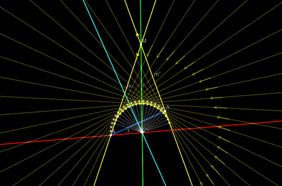
The final advantage of the versor representation is that every rotor has an exponential representation (just as a unit quaternion does).  Since $\mathbf{P}^2=-1$ for a proper point $\mathbf{P}$, the expression $e^{t\mathbf{P}}$ can be evaluated just as if $\mathbf{P}$ were the complex unit $i$, and one obtains $\cos{t} + \sin{t}\mathbf{P}$ as the result.  In fact, when you activate the time slider of the webstart associated to this post (see this post),  the interpolated isometry is calculated using the exponential representation of the motion described here (although of course when it comes to drawing the rotated line, it has to be converted into a matrix and shipped over to the graphics card, which is still living in the old world of vectors and matrices.)

The following figure shows 20 equal steps in the interpolation of the isometry obtained in this way.  The interpolated lines are are drawn as transparent objects to reduce the clutter in the image. You can see that the envelope of the moving line is a circle.

If you’re still with me, I hope that you have gotten a taste of how projective geometric algebra can be a powerful, practical, and elegant tool for doing geometry in a metric-neutral way.

This post builds on the previous one, but returns to the original problem of finding the axis of a hyperbolic isometry.  We show that by using the projective model of hyperbolic geometry one can directly adapt the euclidean solution to obtain the hyperbolic solution also.

The hyperbolic case. The webstart, as explained above, also includes an option to switch the metric to elliptic or hyperbolic We want now to discuss the latter option.  Then the figure includes the unit circle, the boundary of the hyperbolic plane, as the following figure shows:

Does the description of the euclidean construction carry over to the hyperbolic case pictured above?  Clearly there are some constraints on the configuration if there is to be a solution.  For example, the points $\mathbf{A}$ and $\mathbf{A’}$ must be hyperbolic points, and the lines $\mathbf{m}$ and $\mathbf{m’}$ must also be hyperbolic.  But their intersection $\mathbf{M}$ does not need to be hyperbolic; it can be ideal (lie on the unit circle) or also hyper-ideal (lie outside).  Assuming these conditions are met, as they are in the above figure, how does the construction proceed?

The definition of the perpendicular bisector $\mathbf{r}$ is valid.  But what is the angle bisector $\mathbf{c}$ of an angle which, as in this case,  lies outside the hyperbolic disk?  As in the euclidean case, the traditional approach to hyperbolic geometry does not define this.  However, in the projective model one can define it meaningfully.  To do so, one must invoke an involutive correlation $\mathbf{\Pi}$ (a fancy name for a transformation which switches points and lines,  and whose square is the identity) on the projective plane known as the polarity on the metric quadric.  This transformation sends a point $\mathbf{P}$ to the line $\mathbf{P^\perp}$ consisting  of points whose inner product with $\mathbf{P}$ is 0, the orthogonal complement with respect to the hyperbolic metric.

The result is that one obtains a second model of the hyperbolic plane in the exterior of the unit disk, in which the roles of point and line have been reversed.  Then, for example, the point $\mathbf{M}$ when it lies outside the hyperbolic plane, is polar  to the common orthogonal line of $\mathbf{m}$ and $\mathbf{m’}$ inside the hyperbolic disk, and the angle bisector of these two lines is polar to the midpoint of this common orthogonal segment.  Proceeding in this way, one can show that the desired metric properties can be “mirrored” from the exterior of the hyperbolic plane to the interior and hence that the construction given above also solves the given problem for the hyperbolic plane too, although some of the steps may look unfamiliar, since they may involve polar entities, but the metric relations remain unchanged.  A full discussion of this phenomena lies beyond the scope of this post, but hopefully you can get a sense of how the polarity operator in effect produces two hyperbolic planes such that every metric relationship in one is mirrored (with points and lines reversed) in the other.

We leave the same positive conclusion for the elliptic plane for the never-tiring reader.  Here the situation is simplified since there are no real ideal points, every point of the projective plane is also a point of the elliptic plane and any configuration of the initial data is valid, and the construction carried out in the euclidean case goes through here without difficulties.

Having shown that the projective model of these three metric planes provides a reliable basis for solving the construction problem posed in the first post, and doing so in a metric-neutral way, the next post will provide the promised introduction to projective geometric algebra, by giving a (metric-neutral) algebraic formulation of the construction which has formed the content of this and the previous post.

At a student seminar at the TU Berlin in fall 2013, the following problem in plane geometry  was posed, “Given a point lying on a line, and a second point lying on a second line, find the unique direct isometry mapping the first point/line pair to the second.”  The original context was the hyperbolic plane, in thinking about the problem I realized I could solve it in a metric-neutral way, and this blog post and its sequels present that solution. I chose the title since the solution is based on an nifty tool called projective geometric algebra (PGA), and I can’t think of a better introduction to PGA than working out a concrete example like this one.  Buckle your seat belts and enjoy the ride!

What I want to do in this post:

1. Demonstrate an interactive application for playing with this problem.
2. Derive a solution for the problem in the euclidean plane.
3. Discuss some exceptional configurations and show how they can be handled within the context of the projective model of euclidean geometry in a seamless fashion.
4. Indicate how the approach leads to a “cool tool”: projective geometric algebra, a subject for a future post.

I’ve also implemented this result in a jReality webstart application.  If you start this application up, you should see a picture like the following:

Directions for using the webstart. To begin with, you may need to display the control panel to the left of the graphics window. To do this, select the menu item “Window->Left slot” (and deselect “Window->right slot” if you wish).  This is necessary due to a heightened security in Java 7 which prevents correct reading of the built-in property file (which should set these window slots properly.)

If you’re using the webstart application, you can drag any of the three points $\mathbf{A}$, $\mathbf{A’}$ and $\mathbf{M}$ and the diagram adjusts accordingly.  Use the slider labeled time to see how the rotation acts, also to confirm that the rotation actually does what is claimed. Furthermore, to reverse the orientation of either line $\mathbf{m}$ or $\mathbf{m’}$, click on the line; the orientation arrow on the line should flip and the angle bisector $\mathbf{c}$ switches accordingly to the supplementary angle.  Finally, you can switch the metric used using the combo box on the left inspector panel to choose the hyperbolic or elliptic metric also.  The given data remains the same, but the construction is carried out using this metric instead of the euclidean one.  This “metric neutral” capability will be more fully discussed in a later blog.

Return to the geometric problem. Here we want to focus on the challenge of finding a euclidean isometry which moves the point $\mathbf{A}$ to the point $\mathbf{A’}$, and the line $\mathbf{m}$ to the line $\mathbf{m’}$.  (The two lines should be thought of as oriented, so that the orientation is preserved by the isometry.) We claim that the solution is a rotation around point $\mathbf{C}$,  the intersection of line  $\mathbf{r}$ (cyan) and line $\mathbf{c}$ (green). $\mathbf{r}$ is the perpendicular bisector of the segment $\mathbf{AA’}$, while $\mathbf{c}$ is the angle bisector of the angle formed by $\mathbf{m}$ and $\mathbf{m’}$.

Indeed, the center $\mathbf{C}$ of a rotation moving $\mathbf{A}$ to  $\mathbf{A’}$ must lie the same distance to both points, which is the defining condition of $\mathbf{r}$.  Similarly, since the desired rotation maps $\mathbf{m}$ to $\mathbf{m’}$,  the closest point of $\mathbf{m}$ to $\mathbf{C}$ is mapped to the closest point of $\mathbf{m’}$ to $\mathbf{C}$, hence $\mathbf{C}$ lies the same distance to both points.  This condition is satisfied exactly by points on the angle bisector $\mathbf{c}$ of the two lines. (Here one must be careful to specify which angle bisector one means. This depends on the relative orientation of the two lines, and is easy to determine.) Hence the center of the desired rotation must lie on $\mathbf{r}$ and on $\mathbf{c}$, so it is the intersection of these two lines, as shown in the diagram.

Once the center has been found, it´s not hard to express the desired rotation as the composition of two reflections in lines passing through $\mathbf{C}$: first in the line $\mathbf{s}$ (red) followed by reflection in line $\mathbf{r}$ (cyan).  Why does this produce the desired rotation? Clearly reflection in $\mathbf{s}$ fixes $\mathbf{A}$ while that in $\mathbf{c}$ maps $\mathbf{A}$ to $\mathbf{A’}$.  Since $\mathbf{C}$ is fixed by the composition, it must be the rotation we are looking for.  Writing the reflection in line $\mathbf{s}$ as $\mathbf{R_s}$, the rotation is then the composition $\mathbf{R_C} := \mathbf{R_c}\circ \mathbf{R_s}$.

Exceptional configurations. It’s interesting to review the construction for possible exceptional configurations.  For example, $\mathbf{m}$ and $\mathbf{m’}$ may be parallel; then their intersection $\mathbf{M}$ is a so-called point at infinity or, more neutrally,  ideal point.  What is the angle bisector $\mathbf{c}$ in this case?  If the two lines have different orientations (that is, translate one to the other and compare the orientations), then the angle bisector $\mathbf{c}$ is the mid-line, parallel to both, and the construction continues as before.  If not, then $\mathbf{c}$ is the line at infinity itself (!), and the construction continues as before.

Or, $\mathbf{c}$ and $\mathbf{r}$ may be parallel; then their intersection $\mathbf{C}$ is a so-called point at infinity or ideal point, and $\mathbf{s}$, since it goes through $\mathbf{C}$ too, is also parallel to these lines.  Hence the product of the two reflections is not a rotation but a translation.  A bit poetically, one can say, a euclidean translation is a rotation around a point at infinity — by a vanishing angle!

A further exceptional configuration can occur if the lines $\mathbf{r}$ and $\mathbf{c}$ are the same line.  Then they don’t have a well-defined intersection.  It’s not hard to see that this can happen only when $\mathbf{A}$ and $\mathbf{A’}$ lie the same distance from $\mathbf{M}$, so I can rotate $\mathbf{A}$ into $\mathbf{A’}$ by a rotation around $\mathbf{M}$.  Now, if the  orientations of $\mathbf{m}$ and $\mathbf{m’}$ are preserved when I perform this rotation, then it is the desired rotation, and I can construct it by setting $\mathbf{C}$ to $\mathbf{M}$ and continuing as before; if not, the desired rotation center is found by constructing the perpendicular line $\mathbf{a}$ to $\mathbf{m}$ at $\mathbf{A}$; then the intersection of $\mathbf{a}$ and $\mathbf{c}$ is the desired rotation center $\mathbf{C}$ and the construction can continue as before.

Are there other exceptional configurations?  Please post as comment any other ones you find!

The path to geometric algebra. The observant reader will not have missed noting that the correct solution of the exceptional configurations described above proceeded a bit magically.  In particular, finding the correct solution for the first two configurations involved the ideal points and line of the euclidean plane.  These are concepts which are not necessarily associated to euclidean geometry.  That they can be used is due to the discovery by Arthur Cayley and Felix Klein in the 1860’s that projective space can be converted into a metric space in many ways by selecting a quadratic form, the so-called Absolute of the metric space.  Details lie outside the scope of this blog, see my thesis, chapter 4. This Cayley-Klein construction can be directly applied when the quadratic form is non-degenerate, and produces most importantly elliptic (or spherical) and hyperbolic space of any dimension.  It also works for euclidean space, but requires a degenerate quadratic form (some subspaces consist of points with vanishing norm).

For this post, the relevant object is the projective model of the euclidean plane.  Then the points of vanishing norm form a line, the so-called ideal line of the euclidean plane. Parallel lines meet in points of this line. This circumstance allowed us to handle the first two exceptional configurations above, where we sought the intersection of two parallel lines. In almost every euclidean construction or proof there arise such configurations, which have to be handled separately if one is relying of “traditional” euclidean geometry, but which in the context of “projective” euclidean geometry can be handled uniformly. For this reason, the projective model of euclidean geometry has clear advantages over the traditional approach.  In order to carry this out in a rigorous fashion, its useful to translate things into in the correct algebraic setting.

The traditional way of proving that the construction outlined above is correct relies on converting the steps into expressions in vector analysis of the plane.  This approach avoids mention of ideal points and line, and is limited to the euclidean setting.  Is there a better algebraic tool for the job?  In fact, there is a much more comprehensive algebraic structure — which includes vector analysis as a small sub-algebra — such that every step of the above construction can be expressed by a single compact expression. Furthermore, even though the steps of the construction are made based on the euclidean metric, the resulting expressions also provide a correct representation of the same construction when the underlying metric is elliptic or hyperbolic. The differences that arise express naturally the differences between these metrics.  For example, in elliptic space there are no parallel lines. This “metric neutrality” is an expression of  the Cayley-Klein construction underlying this approach. The webstart application allows the user to use these other metrics and confirm that the result is, in fact, metric neutral.

The same comments made regarding the projective model of the euclidean plane apply also to the hyperbolic plane.  Instead of having just one line of ideal elements, in the hyperbolic case there are a circle’s worth of ideal points and lines, and beyond them a second model of hyperbolic geometry, the polar hyperbolic plane, described briefly above. They are not part of the traditional definition of the hyperbolic plane, but can be integrated in an effortless way into the standard model of the hyperbolic plane with the advantage that all projective elements have a significance in hyperbolic geometry, not just the points of the unit disk.  This geometry can also be integrated into the algebraic structure mentioned above.

This algebraic structure is called projective geometric algebra.  I’ll share the details of this algebraic “translation” of our construction problem here in a subsequent post on this blog.