
Let \(\gamma\colon \mathbb S^1 \to \mathbb R^3\) be a closed space curve and \(m\in\mathbb R^3\setminus \gamma(\mathbb S^1)\). The solid angle \(\Omega_{\gamma}(m)\) of \(\gamma\) subtended to the point \(m\) is defined as the (signed) spherical area enclosed by the projection \(\hat\gamma\) of \(\gamma\) to the unit sphere with center \(m\),\[\hat\gamma = \frac{\gamma-m}{|\gamma – m|}+m\] Note that the spherical area is defined only up to addition of an integral multiple of \(4\pi\). Hence \(\Omega_\gamma\) is a well-defined angle-valued map\[\Omega_\gamma\colon \mathbb R^3\setminus \gamma(\mathbb S^1) \to \mathbb R/4\pi \mathbb Z.\]The solid angle of a closed discrete space curve \(\gamma\colon \mathbb Z/n\mathbb Z \to \mathbb R^3\) is then defined by the solid angle of the closed polygon \(P_\gamma\) corresponding to \(\gamma\).
The polygon \(P_\gamma\) projects to the spherical polygon corresponding to \((\gamma-m)/|\gamma – m|+m\). Since translations do not change area we are left with the problem to compute the (signed) area of a spherical polygon in the unit sphere \(\mathbb S^2\subset \mathbb R^3\). This can be done e.g. by the Gauss-Bonnet Theorem: Let \(\hat\gamma \colon \mathbb Z/n\mathbb Z \to \mathbb S^2\). Let \(\mathbb D\) be the unit disk in \(\mathbb R^2\) and \(f\colon \mathbb D \to \mathbb S^2\) be a regular surface such that \(f|_{\mathbb S^1}\) parametrizes the spherical polygon corresponding to \(\hat\gamma\). Then, since the all edges are geodesics and \(\chi_M = 1\), we get\[\mathrm{Area}(f) = \int_D f^\ast d\mathrm{vol}_{\mathbb S^2} = 2\pi – \sum_i\kappa_i,\]where \(\kappa_i\) denote the kink angles of the spherical polygon. \(\kappa\) can be computed from the discrete spherical curve \(\hat\gamma\).
Another, more elementary way to compute the area is to use a triangulation. Therefore choose a point \(c\in\mathbb S^2\setminus\{-\hat\gamma_0,\ldots,\hat\gamma_{n-1}\) and connect each vertex of \(\hat\gamma\) to \(c\) by the great circle arc of length \(< \pi\). Note that the points \(c\), \(\gamma_i\) and \(\gamma_{i+1}\) lie in an open hemisphere. We obtain a triangulated disk with \(n\) triangles of the form \(\triangle_i = (c,\hat\gamma_i,\hat\gamma_{i+1})\) each of which is contained in an open hemisphere. The area enclosed by \(\hat\gamma\) is then just the sum of the areas of the spherical triangles \(\triangle_i\) for which we have an elementary formula: Given a positively oriented spherical triangle \(\triangle = (a_0,a_1,a_2) \in \mathbb S^2\) contained in an open hemisphere, then the area\[\mathrm{Area}(\triangle) = \sum_{i=0}^2 \alpha_i – \pi,\]where \(\alpha_i\in (0,\pi)\) denotes the interior angle at \(a_i\). To see this look at the lunes \(\lambda_i\) generated by \(a_{i-1}\), \(a_{i}\) and \(a_{i+1}\).
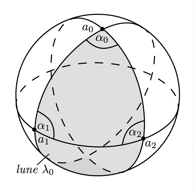
Then the union of \(\lambda_0\), \(\lambda_1\) and \(\lambda_2\) covers half of the sphere. Thus the area of their union is \(2\pi\). Each lune itself has area \(2\alpha_i\). Thus we get \(2 \sum_{i=0}^2 \alpha_i = 2\pi + 2\mathrm{Area}(\triangle)\). If the original triangle was negatively oriented we just flip the sign.
Yet another way to compute the area of an oriented spherical triangle is to use the following relation between parallel transport and curvature: Let \(M\) be a Riemannian surface with boundary \(\partial M\), let \(J\) denote the complex structure of \(M\) (i.e. the 90 degree rotation in \(TM\)) and let \(P_\eta\) denote the parallel transport along a curve \(\eta\) in \(M\). Then\[P_{\partial M} = e^{J\int_M K\,d\mathrm{vol}_M}.\] In particular, if \(K=1\), we get\[P_{\partial M} = e^{J\mathrm{Area}(M)}.\]The advantage of this version is that is also applies to singular triangles.
Consider two point \(p\) and \(q\) on \(\mathbb S^2 \subset \mathbb R^3 \cong \mathrm{Im}\,\mathbb H\). If \(q\neq -p\), then there is a unique shortest great circle arc \(\eta\colon [0,1]\to \mathbb S^2\) connecting them. So we can speak of \(P_{p,q}\). Actually \(P_{p,q}\) can be written down by quaternions:\[P_{p,q}(X) = \psi_{p,q} X \psi_{p,q}^{-1}.\]Let us verify that \(\psi_{p,q} = q(p+q)\): The quaternion \(p+q\) represents a \(180\) rotation \(R_1\) around the vector \(p+q\). Similarly, \(q\) represents a \(180\) degree rotation \(R_2\) around \(q\). Thus \(\psi_{p,q}\) representing the rotation \(R_2R_1\) restricts to an isometry \(T_p\mathbb S^2 \to T_q\mathbb S^2\) mapping \(\eta^\prime(0)\) to \(\eta^\prime(1)\). Since \(\eta\) is a geodesic, \(\eta^\prime\) is parallel. The claim then follows since parallel transport is angle and orientation preserving.
The quaternion \(\psi_{p,q}\) is defined only up to a non-zero real multiple. Thus, if \(p=q\), then \(\psi_{p,q} = 1\). If \(p\neq q\), then \[\psi_{p,q} = 1+\tan(\mathrm{dist}(p,q)/2)\, N,\] where \(\mathrm{dist}(p,q)\) denotes the spherical distance of \(p\) and \(q\), i.e. the length of \(\eta\), and \(N\) denotes the normal of the great circle arc pointing to the left, i.e. \(N = J\eta^\prime(t)\) for some \(t\).
Now, let us consider the spherical triangle \(\triangle = (a_0,a_1,a_2)\). We have \[e^{J\mathrm{Area(\triangle)}} = P_{a_2,a_0}\circ P_{a_1,a_2}\circ P_{a_0,a_1}.\]
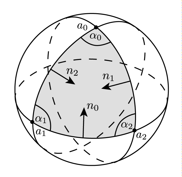
In quaternions this becomes\[\rho\,(1+\tan(\mathrm{Area}(\triangle)/2)a_0) = (1+\tan(\ell_1/2)n_1)(1+\tan(\ell_0/2)n_0)(1+\tan(\ell_2/2)n_2).\]Here \(\ell_i\) denotes the arc length and \(n_i\) the inward pointing normal of the great circle arc opposite to the point \(a_i\). We can multiply the equation from the right by the inverse of \(1+\tan(\ell_2/2)n_2\). This yields the following quaternionic equation\[\rho\,(1+\tan(\mathrm Area(\triangle)/2)a_0)(1-\tan(\ell_2/2)n_2) = (1+\tan(\ell_1/2)n_1)(1+\tan(\ell_0/2)n_0),\] where the real factor \(|1+\tan(\ell_2/2)n_2|^{-2}\) is absorbed into \(\rho\).
Sicne \(a_0\perp n_2\), taking now the real part on both sides of the quaternionic equation yields\[\rho = 1 – \tan(\ell_0/2)\tan(\ell_1/2)\langle n_0,n_1\rangle = 1 + \tan(\ell_0/2)\tan(\ell_1/2)\cos(\alpha_2).\]By taking the imaginary part on both sides of the quaternionic equation, we get\begin{gather*}\rho(\tan(\mathrm{Area}(\triangle)/2)a_0 – \tan(\ell_2/2)n_2 – \tan(\mathrm{Area}(\triangle)/2)\tan(\ell_2/2)a_0\times n_2)\\ = \tan(\ell_0/2)n_0 + \tan(\ell_1/2)n_1 – \tan(\ell_0/2)\tan(\ell_1/2)n_0\times n_1.\end{gather*} Moreover, \(a_0\perp n_1,n_2\) and \(n_0\times n_1 = \sin(\alpha_2) a_2\), where \(\alpha_i\) denotes the oriented interior angle at \(a_i\). If we now build the scalar product with \(a_0\), we obtain \[\rho\tan(\mathrm{Area}(\triangle)/2) = \tan(\ell_0/2)\bigl(\langle a_0,n_0\rangle – \tan(\ell_1/2)\sin(\alpha_2)\cos(\ell_1)\bigr).\]With \(\sin(\ell_0)\langle n_0,a_0\rangle = \langle a_1\times a_2, a_0\rangle = \sin(\ell_0)\sin(\ell_1)\sin(\alpha_2)\) we then get\begin{gather*}\langle a_0,n_0\rangle – \tan(\ell_1/2)\sin(\alpha_2)\cos(\ell_1) = \sin(\alpha_2)\bigl(\sin(\ell_1)- \tan(\ell_1/2)\cos(\ell_1)\bigr) \\ = \sin(\alpha_2)\bigl(2\sin(\ell_1/2)\cos(\ell_1/2) – \tan(\ell_1/2)(\cos^2(\ell_1/2) – \sin^2(\ell_1/2)\bigr) \\ = \sin(\alpha_2)\tan(\ell_1/2)\bigl(2\cos^2(\ell_1/2) – (\cos^2(\ell_1/2)-\sin^2(\ell_1/2)\bigr) = \sin(\alpha_2)\tan(\ell_1/2).\end{gather*}Hence we get\[\tan(\mathrm{Area}(\triangle)/2) = \frac{1}{\rho}\tan(\ell_0/2)\tan(\ell_1/2)\sin(\alpha_2) = \frac{\tan(\ell_0/2)\tan(\ell_1/2)\sin(\alpha_2)}{1 + \tan(\ell_0/2)\tan(\ell_1/2)\cos(\alpha_2)}.\]Moreover, note that the tangents are given by purely algebraic formulas: Since \(\tan(\theta/2) = \sin(\theta)/(1+\cos(\theta))\) we have \[\tan(\ell_0/2) = \frac{|a_0-\langle a_0,a_2\rangle a_2|}{1 + \langle a_0,a_2\rangle},\quad \tan(\ell_1/2) = \frac{|a_1-\langle a_1,a_2\rangle a_2|}{1 + \langle a_1,a_2\rangle}.\]Moreover, \[\cos(\alpha_2)\sin(\ell_0)\sin(\ell_1) = \bigl\langle a_0 – \langle a_0,a_2\rangle a_2, a_1 – \langle a_1,a_2\rangle a_2\bigr\rangle = \langle a_0,a_1\rangle – \langle a_0,a_2\rangle\langle a_2,a_1\rangle\] and with \(\det(a_0,a_1,a_2)=\sin(\ell_0)\sin(\ell_1)\sin(\alpha_2)\) we get\[\alpha_2 = \mathtt{atan2}(\det(a_0,a_1,a_2),\langle a_0,a_1\rangle – \langle a_0,a_2\rangle\langle a_2,a_1\rangle).\]
Now, given a closed discrete space curve \(\gamma\) we can compute the solid angle \(\Omega_\gamma(m)\). But how can we visualize the solid angle in Houdini?
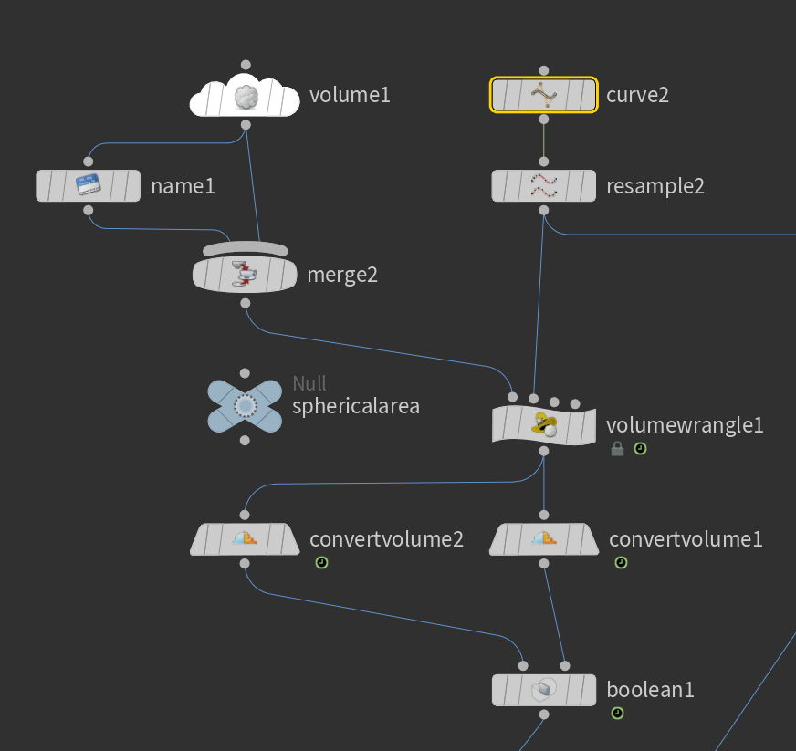
A convenient way to do this is to compute the solid angle for the voxel centers of a volume surrounding \(\gamma\) and then use a convert volume node to extract the zero level set of \(\Omega_\gamma\). Here is how such a network may look like.
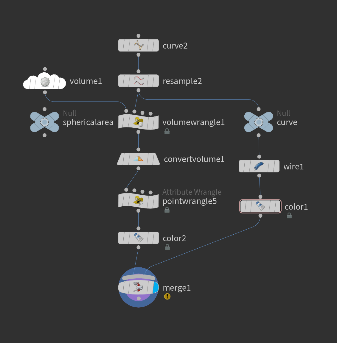
Volume wrangle nodes work quite similar to attribute wrangle nodes. Here the code block of the node volumewrangle1 in the network above:
|
1 2 3 4 5 6 7 8 9 10 11 12 13 14 15 |
// import method to compute solid angle `chs("../sphericalarea/code")` // write curve to vector array int n = npoints(1); vector P[]; for(int i=0; i<n; i++){ P[i] = point(1,"P",i); } // read of coordinate of the voxel center vector m = v@P; float Omega = solidAngleOfCurve(P,m); // write Omega to the volume with name Omega f@Omega = Omega; |
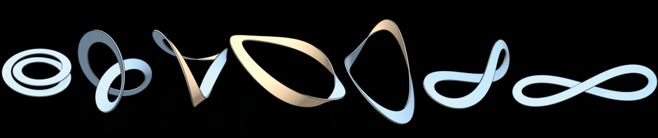
The method to compute the solid angle is contained in a string parameter of a null node ‘sphericalarea’ and imported at the beginning of the block. The volume is initialized with the name Omega (the string specified in the name field of the volume node). The values then can be accessed and set via f@Omega. Note that volumes also have a boundary type which here should be set to ‘streak’. You find this parameter in the properties tab of the Volume node. Here is what we get.
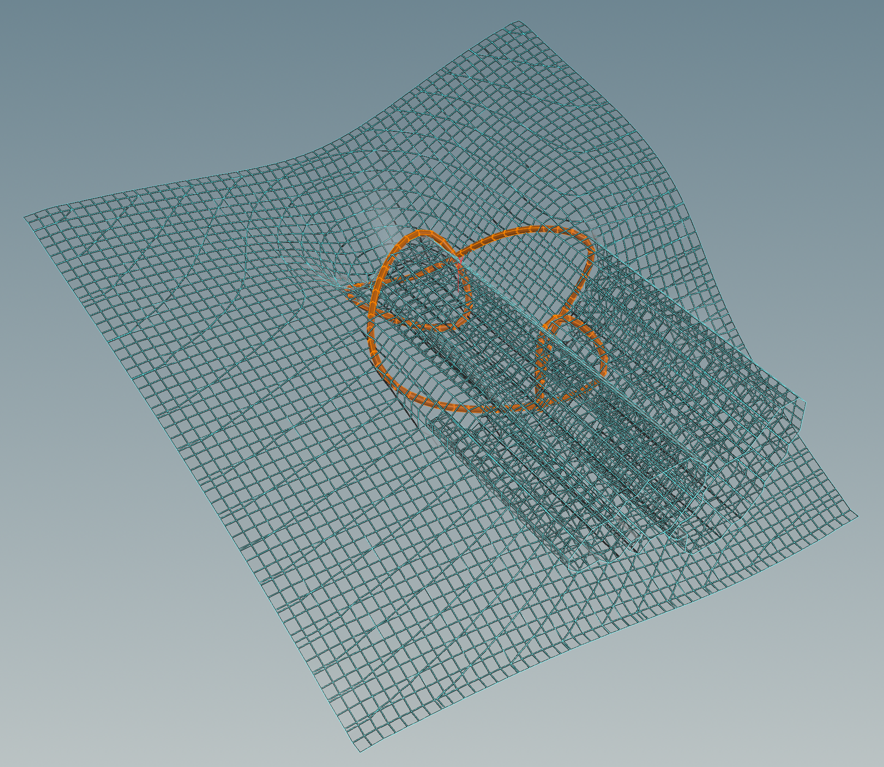
The artifacts in the picture above are due to \(4\pi\) jumps , which cannot be handled by the convert volume node. We can get rid of them by applying a \(4\pi\)-periodic function as e.g. \(x\mapsto \sin(x/2)\). Only that the zero set now corresponds to \(\Omega_\gamma^{-1}(0)\cup \Omega_\gamma^{-1}(\pi)\). We can remove the \(\Omega_\gamma^{-1}(\pi)\) part as follows: Create a second volume to store the values of \(\cos(\Omega_\gamma/2)\). From this we extract a second surface and use a boolean intersect node to cut of everything inside the second surface.
Homework (due 26 June). Write a network that computes for a given discrete space curve the level sets of the solid angle.