What is the most powerful thing in the universe? Perhaps nobody knows, but in our world it might either be stokes theorem or the Laplace operator. It is shocking how many algorithms we end up dealing with the Laplace operator in its core steps. Chances are good that whatever you do with the knowledge of these tutorials will require the Laplace operator in some form.

In this tutorial, we shall build the cotan-Laplace operator to compute a minimal surface given a fixed boundary. Since this is a technical tutorial we will leave out the theoretical reasoning behind this. However, we will show you how to build the sparse matrix since it requires detailed technical knowledge of the relationships between points, vertices and primitives to build a sparse matrix using scipy.

 

The Input Geometry

To compute a minimal surface we need a starting surface with the topology that we shall use. In our case we will keep things simple and use a disc mesh that we will deform into some random shape. Here we display how our shape was made:

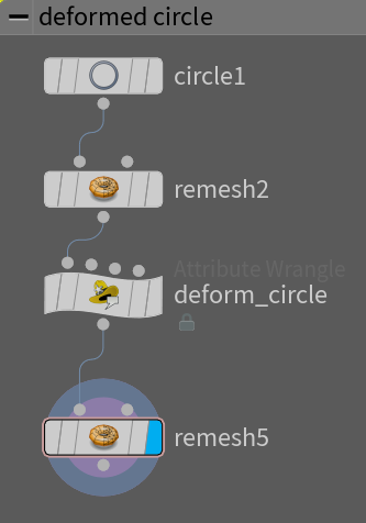
With the following code in the deformation:

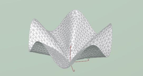
That results in this LA tostada shape:

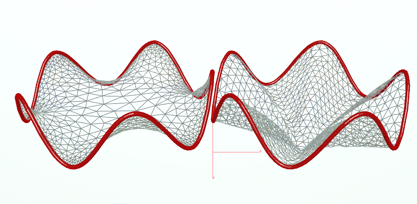
We can also start with other shapes such as the two following ones:

 

The Surface Minimization Algorithm

Now we get to the complicated part which we will guide you through.

Iteration Control

Our method is an iteration that can be implemented using an Block Begin – Block End pair of nodes. The complicated part of the algorithm will be put in a subnet in between that we call “Reduce Surface Area”.

Note that we can use a clever trick to quickly edit the number of iterations. In the block end node, simply replace the “Iterations” field with $F so that you can edit this field using your keyboard from anyplace in Houdini just as you would normally edit the frame number.

Inside the Subnet we will have a network looking like this:

Python Preparations

At first we remesh the node and then make some preparations for python. We create attributes for the point Ids and for the positions.

Now we have to come up with a more complicate enumeration scheme. Our sparse Laplace matrix will have the number of rows and columns equal to the number of points and values will be assigned to the diagonals but also the $i$th row and $j$th column entry will be written into whenever there is an edge connecting the $i$th point with the $j$th point. How can we collect these values fast? Here is one way to do it: for every triangle collect the point ids of the 3 points around it and store them into a attribute vector resting on the primitive. Not just one vector, but two vectors as computed by the following code.

Explanation: The $k$th entry ( $k\in\{1,2,3\}$ ) of the start vector indicates from where an edge starts while the $k$th entry of the end vector indicates where that exact same edge ends. Now our code looks like this:

Marking the Boundary

Next we want to label each boundary point using an attribute. A magical Houdini trick to archive that involves the group node. This allows us to name a group for a specific selection of conditions (or manual selection with the mouse). In our case, we can group together the edges and mark the option unshared edges. Boundary edges are unshared edges and thus the right points are grouped together in a group that we name boundary.

Next we can add a point wrangle that only runs on the group: boundary. This way we can set an integer boundary attribute equal to 1 only for boundary points.

Next we have to set the function g equal to zero everywhere but on the boundary. This is done in favor of the algorithm that we use and is done with the following point wrangle code:

The Making of the Sparse Laplace Matrix

Now we will focus on creating the Laplace matrix. Sparse matrices require 4 details to be constructed.

• The dimension of the matrix: in our case the number of points.
• An array of row indices of non zero entries.
• An array of column indices of non zero entries corresponding to the above row indices.
• An array of values corresponding to the row/column index pair.

Let us try to compute the values for the matrix. The first thing we have to do is to compute edge lengths. We do this by iterating over the vertices as the number of vertices is equal to the number of half edges and Houdini does not iterate over the edges.

Next we compute the cotan values on every vertex.

Now that we have all the cotan weights ready, we only need to collect them in a reasonable way for python to grab them. For the off-diagonal entries we will grab the 3 cotan weights around each triangle and store them in one vector inside the triangle. Notice that we store the edge related cotan values inside the attribute vector in the exact same order as we have stored the start and end vector point indices in order to correctly relate the edges with their cotan value in the sparse matrix later.

The diagonal entries of the cotan-Laplace operator depend on all other entries in the row/column and we have one diagonal entry per point. This is why for the diagonal entries we will grab a point wrangle node and visit all the neighbours of each point to sum up the cotan weights.

And at last we have everything ready to really build the cotan-Laplace matrix inside python.  In the next python node we will collect all the needed attributes from the points and the primitives that we have just created. For the Off-diagonal part of the sparse matrix creation we grab the indices from the start and end vectors and the corresponding values from the omega vector on the primitives. For the diagonal entries we grab the point indices with the attributes we just saved on the points.

 

Solving the Poisson Equation

Next we will show how the Poisson equation $\Delta f=g$ can be solved inside a python node.

First we will read the function g into python (we had stored it as float attributes gx,gy,gz and we then cache them into python.

And next we take another python node, read all the inputs g and the Laplace matrix in and solve the Poisson equation.

And at very last we copy the computed values into the point positions using a point wrangle node.

Displaying the Results

We want to display the results using soap films with highlighted boundary. Here we present a simple way how to make that possible.

To highlight the boundary we label every boundary point again and then use that information in a detail attribute wrangle node in order to loop over each vertex (thus over each edge) and add a line segment to that edge if it is a boundary edge.  The fuse node afterwards then takes care of fusing two points from different line segments into one point. This way we actually have a complete polygonal line for every boundary component. Here is the code for the creation of the boundary lines. For the textures please look at the texture tutorial.

The results looks as follows:

Note that if you make the tube too long  the minimal surface has to split the mesh into two discs. However, our implementation does not yet handle such geometry splittings.

 

Just to clear things up, this is how our final network looks like: