
This post is also meant as a first introduction to using Houdini.
In most applications discrete curves and surfaces are used as approximate descriptions of smooth objects. This situation is close in spirit to Numerical Analysis where the discrete objects would be considered as approximations by “finite elements” of some smooth geometry.
In Discrete Geometry the polyhedral surfaces themselves are the prime focus of study. The emphasis here is often on questions of combinatorics and many arguments have the flavor of Elementary Geometry.
Also in Discrete Differential Geometry the discrete objects are studied in their own right. However, the goal is to develop a theory that corresponds as closely as possible to the theory of smooth curves and surfaces. Questions of convergence in the continuum limit are still marginally interesting. They are however not as central as they would be in in Numerical Analysis. In Discrete Differential Geometry the question remains interesting how the theory performs if the discrete objects have only very few vertices.
Both in the context of Discrete Geometry and the context of Discrete Differential Geometry the wish sometimes arises to render discrete curves and surfaces in a way that gives more prominence to individual vertices, edges and faces:
- In classical geometry drawings it is customary to draw distinguished points as small circles. The analog of this in a computer-aided three-dimensional context is to display points as small spheres.
- The orientation of straight lines in three dimensions becomes much more clearly evident if the line is drawn as a thin cylindrical tube with appropriate lighting.
- The spatial orientation of planar faces is easier to discriminate if appropriate lighting is applied.
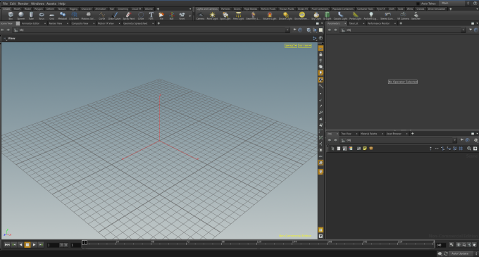
Let us start with the facets. Start up Houdini and create a Geometry node. To this end make sure the focus is in the node editor window (bottom right) and hit the Tab key. A menu with a list of all available node typed will pop up. Start typing “g” and you will see a list of all node types whose name starts with “g”. If you go on typing to complete the name “geometry”, already after one more keystroke the choice will narrow down to a unique one. Now you can either hit the Enter key or click on the only remaining menu item labeled “Geometry”. A rectangular outline will appear in the Network View that allows you to place the node at a position of your choice. As soon as it is placed the parameter editor window above will show the parameters associated with the currently highlighted node in the network editor.

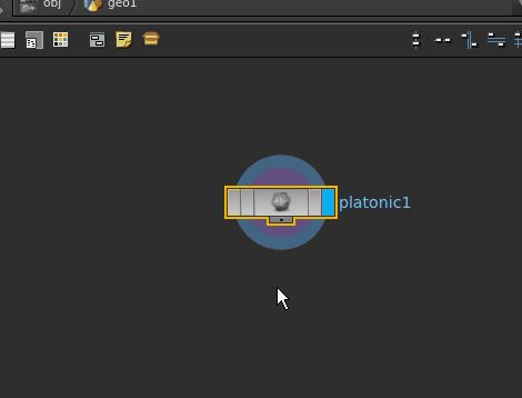
Dive into the newly created geometry node by double-clicking on it. Inside you will find a node providing the standard test geometry. Select it by clicking on it and delete it by using the Delete key. Instead of the standard geometry we will attach a geometry of our choosing. To do so, create a node of type Platonic Solids. Once again do this by hitting Tab and starting to type “Plato…” and place the node. In the upper right panel of the Houdini window (the parameter window) you will see the parameters associated with the Platonic solid node.
Use the dropdown menu labeled “Solid Type” to select “Cube.”
If you make sure that the camera symbol visible on the left vertical toolbar (left of the scene view window) is selected, you can rotate the whole scene (actually you rotate the camera) using the left mouse button and translate it using the middle mouse button. You can toggle the grid on or off by clicking on the uppermost symbol on the right (of the scene view) vertical toolbar.
NOTE: Houdini 16 has updated the normals on the platonic solids. The fix for the strange effect is not necessary anymore here. However, be sure to read about it as your own creations might still have these effects.
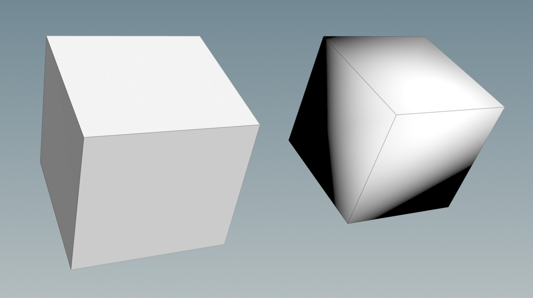
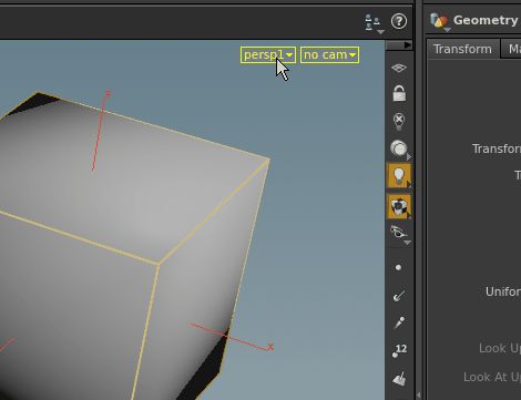
The lighting of this cube seems strange. The reason is that by default Houdini treats all discrete surfaces as approximations to smooth ones, so it is only natural to treat the cube as a coarse approximation to something like a round sphere. This becomes more apparent if we show the normals: From the yellow menu in the upper right of the Scene View labeled “persp1” choose “Display” and make a checkmark next to “Normals” (alternatively find the “display normals” icon button on the right vertical tool bar in the scene view window).
Normals are interpolated across the surface for shading purposes. Here we see that the cube has only a single normal at each vertex. On the other hand, the cube on the left shows three different normals at each vertex, one for each adjacent face. This is what we want. So we have to find a way to tell Houdini that we really mean a surface with planar faces which make sharp angles.
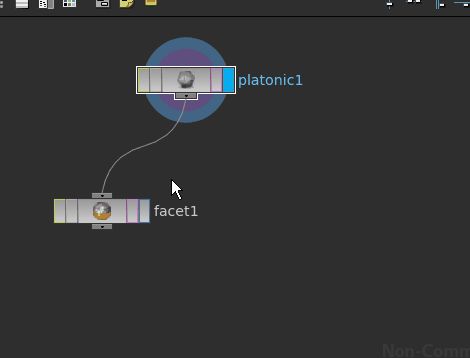
We can achieve this by placing a node of type Facet below the Platonic Solids node. Same as before: be sure focus is in the network editor window, hit TAB and start typing “Fac…” After placing the box connect the output of the node of type Platonic Solids to the input of the node of type Facet: Click on either port with the left mouse button, release the button, move over to the other port and click again.
In the upper right corner the parameter interface of the Facet node is accessible. There check Cusp Polygons, which means that all edges between faces that make an angle bigger that the Cusp Angle displayed right below will be treated as sharp angles. 20 degrees (the default number already there) would be small enough for the cube, but we might as well type in zero here. By this we indicate that all edges between faces are to be treated as sharp edges. So far you don’t see any change in the Scene view. This is because the “Display/Render” button is highlighted still in the “platonic” box (it is the rightmost blue rectangle in that block). Now click on the rightmost rectangle on the Facet node in order to make it the current Display node. Now we see the cube with the shading that we intend.
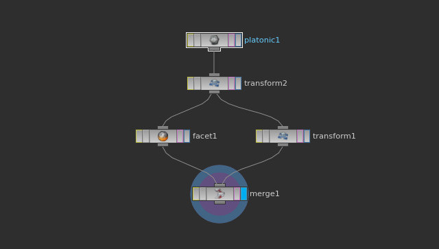
In order to make the pictures shown above we placed the original cube side by side by its faceted version. For this we used two nodes of type Transform to rotate the original cube and to translate one version of it. These transformations can be typed into the parameter windows (useful when you want precise values), or they can be chosen interactively. For the latter, select one of the transforms. Then in the Scene View select the “Show Handle” button. Play with the handle that comes up. It will allow for constrained and free hand motions. In the end we used a node of type Merge in order to combine the two resulting cubes in one single object:
Notice that you will see different things in the Scene view depending on which node has the blue box checked. Also play with the parameters in each node.
written by Pinkall/Padilla 2016/17
