As I used various $\LaTeX$ commands and shortcuts which are not available here, I will not upload lectures 26 and 27 into the blog.
Yet they are included in the pdf version of the lecture notes which is available here.
Lectures 26 and 27
Reply
As I used various $\LaTeX$ commands and shortcuts which are not available here, I will not upload lectures 26 and 27 into the blog.
Yet they are included in the pdf version of the lecture notes which is available here.
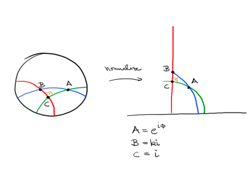
Theorem (Hyperbolic Pythagoras).
Let $\triangle ABC$ be a hyperbolic triangle with angles $\alpha$, $\beta$ and $\gamma=\frac\pi2$.
Then the lengths of the edges $a$, $b$ and $c$ satisfy
\[\cosh c=\cosh a\cdot\cosh b\,.\]
Proof.
We calculate the length in the upper half-plane model after normalizing the triangle to the following:
We use the formula derived for the hyperbolic distance in the upper half-plane using complex variables:
\[
\cosh d(z_1,z_2)-1
=\frac{\lvert z_1-z_2\rvert^2}{2\operatorname{Im}z_1\operatorname{Im}z_2}\,,
\]
So for the length of the edges of the triangle we obtain:
\begin{align*}
\cosh a&=1+\frac{\lvert B-C\rvert^2}{2\operatorname{Im}B\operatorname{Im}C}\\
&=1+\frac{(k-1)^2}{2k}=\frac{k^2+1}{2k}\\
\cosh c&=1+\frac{\lvert\mathrm e^{\mathrm i\phi}-k\mathrm i\rvert^2}{2k\sin\phi}\\
&=1+\frac{\left(\mathrm e^{\mathrm i\phi}-k\mathrm i\right)\left(\mathrm e^{-\mathrm i\phi}+k\mathrm i\right)}{2k\sin\phi}\\
&=1+\frac{k^2+1-2k\sin\phi}{2k\sin\phi}\\
&=\frac{k^2+1}{2k\sin\phi}\\
\cosh b&=\frac{1^2+1}{2\cdot1\cdot\sin\phi}\\
&=\frac1{\sin\phi}\,.
\end{align*}
This calculation implies the required equality.
What is the relation of hyperbolic and Euclidean triangles?
Looking at “small” hyperbolic triangles (i.e. triangles with small edge lengths and area) hyperbolic triangles behave similar to Euclidean triangles.
If the area is very small, then the sum of its interior angles is almost $\pi$.
The hyperbolic Pathagoras’ Theorem becomes the Euclidean Pythagoras’ Theorem for small edge lengths:
The Taylor series for $\cosh$ is $\cosh x=\sum\frac{f^{(k)}(0)}{k!}x^k=1+\frac12x^2+\dotsb$.
Thus $\cosh c=\cosh a\cdot\cosh b$ becomes
\[1+\frac{c^2}2+\dotsb=\left(1+\frac{a^2}2+\dotsb\right)\left(1+\frac{b^2}2+\dotsb\right)\,,\]
hence
\[1+\frac{c^2}2=1+\frac{a^2}2+\frac{b^2}2+\underbrace{\frac{a^2b^2}4+\dotsb}_{\approx0}\]
which gets $c^2=a^2+b^2$ for small $a$, $b$ and $c$.
Consider the following maps:
\[g\colon\hat\C\to\hat\C\,,\ z\mapsto\frac{az+b}{cz+d}\,,\]
where $ad-bc>0$ and $a,b,c,d\in\R$.
Here, $g$ maps $\infty$ to $\frac ac$ and $-\frac dc$ to $\infty$.
Also,
\[\tilde g\colon\hat\C\to\hat\C\,,\ z\mapsto\frac{-a\bar z+b}{-c\bar z+d}\,.\]
Theorem.
An arbitrary hyperbolic isometry of $H_+^2$ is of the form
\[z\mapsto\frac{az+b}{cz+d}\quad\text{or}\quad z\mapsto\frac{-a\bar z+b}{-c\bar z+d}\,,\]
where, again, $ad-bc>0$ and $a,b,c,d\in\R$.
Proof.
Let $\phi\colon H_+^2\to H_+^2$ be an isometry. We can construct a map $g$ which is one of the following, such that $g\circ\phi$ maps the imaginary axis onto itself and $g\circ\phi(\mathrm i)=\mathrm i$ and $g\circ\phi((0,\mathrm i))=(0,\mathrm i)$:
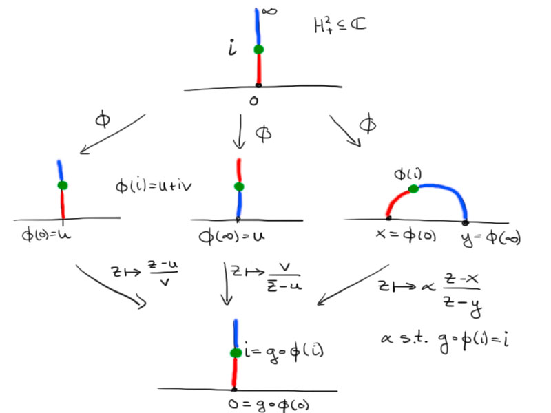
Then $g\circ\phi$ is an isometry, since $g$ and $\phi$ are. Further $g\circ\phi$ is the identity on the imaginary axis, as it is isometric and maps the imaginary axis onto itself preserving the intervals $(0,\mathrm i)$ and $(\mathrm i,\infty)$.
Now consider $x+\mathrm i y$ with $g\circ\phi(x+\mathrm i y)=u+\mathrm i v$.
We have $d(k\mathrm i,x+\mathrm i y)=d(g\circ\phi(k\mathrm i),u+\mathrm i v)=d(k\mathrm i,u+\mathrm i v)$ for all $k\in\R^+$.
Thus
\[\frac{\lvert k\mathrm i-(x+\mathrm i y)\rvert^2}{2ky}=\frac{\lvert k\mathrm i-(u+\mathrm i v)\rvert^2}{2kv}\]
and hence
\[(x^2+(k-y)^2)v=(u^2+(v-k)^2)y\]
for all $k$.
This implies $y=v$ and $u=\pm x$.
So $g\circ\phi$ is either the identity or it the reflection with respect to the imaginary axis, $z\mapsto-\bar z$.
As $\phi=g^{-1}\circ g\circ\phi$, $\phi$ is of the given type.
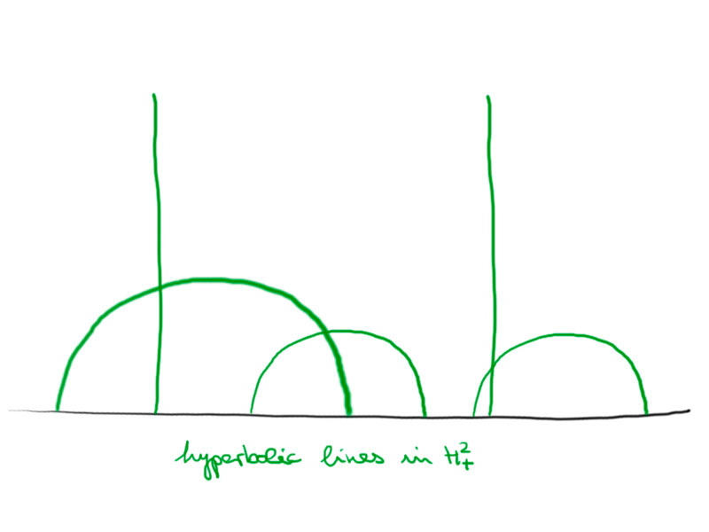
Lengths/distances in $H_+^2$.
Two points $P_1$ and $P_2$ in the upper half-plane model either have the same $x$ coordinate or not. If they share the $x$ coordinate the geodesic through two points is a straight line. Otherwise it is a semi-circle. Let us calculate the hyperbolic distance between two points depending on the two cases.
Case 1.
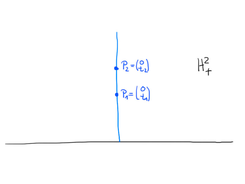
\[
\gamma\colon[t_1,t_2]\to H_+^2\,,\ \gamma(t)=\begin{pmatrix}0\\t\end{pmatrix}\,.
\]
\begin{align*}
d(p_1,p_2)&=\int_{t_1}^{t_2}\sqrt{g_{\gamma(t)}\left(\begin{pmatrix}0\\1\end{pmatrix},\begin{pmatrix}0\\1\end{pmatrix}\right)}\mathrm dt \\
&=\int_{t_1}^{t_2}\frac1t\sqrt{\left(\begin{pmatrix}0\\1\end{pmatrix},\begin{pmatrix}0\\1\end{pmatrix}\right)}\mathrm dt=\log\frac{t_2}{t_1}\,.
\end{align*}
So the length/distance only depends on the ratio $\frac{t_2}{t_1}$, not on the values.
Case 2.
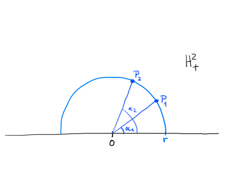
\begin{align*}
P_1&=r\begin{pmatrix}\cos\alpha_1\\\sin\alpha_1\end{pmatrix}&
P_2&=r\begin{pmatrix}\cos\alpha_2\\\sin\alpha_2\end{pmatrix}\,.
\end{align*}
Here,
\[\gamma\colon[\alpha_1,\alpha_2]\to H_+^2\,,\ \gamma(\alpha)=r\begin{pmatrix}\cos\alpha\\\sin\alpha\end{pmatrix}\,.\]
By this we get
\[d(p_1,p_2)=\int_{\alpha_2}^{\alpha_1}\frac1{\sin t}\mathrm dt=\left.\log\tan\frac t2\right\vert_{\alpha_1}^{\alpha_1}=\log\frac{\tan\frac{\alpha_1}2}{\tan\frac{\alpha_2}2}\,,\]
i.e. the distance depends on the angle, not on the radius.
Remrk.
The following maps are isometries of $H_+^2$:
Both transformations leave the Riemmanian metric invariant.
Proposition.
The distance in the Poincaré halfplane model $H_+^2\subset\C$ between two points $z_1$, $z_2$ is given by
\[\cosh d(z_1,z_2)-1=\frac{\lvert z_1-z_2\rvert^2}{2\operatorname{Im} z_1\operatorname{Im} z_2}\,.\]
Proof. Calculation using some trigonometric identities.
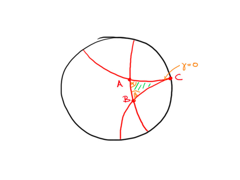
Let $A$, $B$, $C$ be three points in the hyperbolic plane $H^2$ not all on one line.
Then the hyperbolic triangle is given by
\[\triangle ABC=\{\lambda A+\mu B+\nu C:\lambda,\mu,\nu>0\}\cap H^2\,.\]
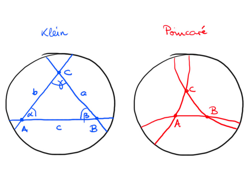
The triangle defined by $A$, $B$, $C$ in the Klein model is
\[\triangle ABC=\{\lambda A+\mu B+\nu C:\lambda,\mu,\nu\geq0,\lambda+\mu+\nu=1\}\,.\]
We label the vertices, angles and sides of a triangle as shown in the above picture.
Observation: $\alpha+\beta+\gamma<\pi$ for any hyperbolic triangle.
Consider a triangle in the Poincaré disc. We may use a hyperbolic motion to move $A$ to the center of the disc.
The angles between the hyperbolic lines at $B$ and $C$ are smaller than the angles of the Euclidean triangle, hence $\alpha+\beta+\gamma<\pi$.
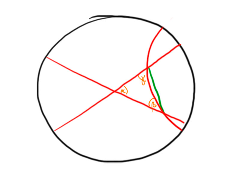
Proposition.
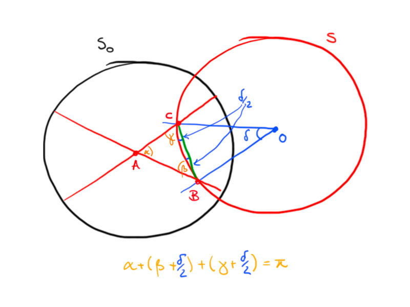
For $\alpha,\beta,\gamma>0$ with $\alpha+\beta+\gamma < \pi$ there exists a hyperbolic triangle. The triangle is unique up to hyperbolic motions.
Proof. We proof the proposition by construction: Let $\delta > 0$ such that $\alpha+\beta+\gamma+\delta = \pi$. Construct a Euclidean triangle with angles $\alpha$, $\tilde\beta = \beta+\delta/2$ and $\tilde\gamma=\gamma+\delta/2$. Then construct a circle $S$ through $B$ and $C$ such that $\angle OBC=\delta$ and $O$ on the other side of $a$ than $A$. The angles between $S$ and $b$, $c$ are $\beta$ and $\gamma$, resp. Now, construct a circle $S_0$ centered in $A$ which intersects $S$ orthogonally. Scaling this construction such that the second circle has radius $1$ yields a triangle with the prescribed angles in the Poincaré model.
Theorem.
The area of a hyperbolic triangle with angles $\alpha$, $\beta$, $\gamma$ is $\pi-(\alpha+\beta+\gamma)$.
Proof.
Consider a triangle with one point at infinity, i.e. on the boundary of the disc in the Poincaré model.
We may normalize the picture and transform it to the upper half-plane model, such that we obtain the following picture:
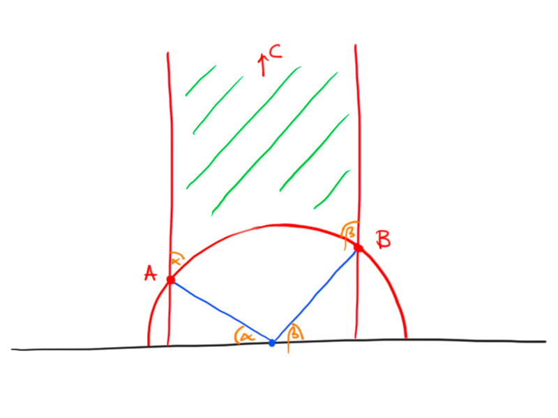
The area of the triangle is
\begin{align*}
T(\alpha,\beta,0)&=\int_{-\cos\alpha}^{\cos\beta}\int_{\sqrt{1-x^2}}^\infty\frac1{y^2}\mathrm dy\mathrm dx \\
&=\int_{-\cos\alpha}^{\cos\beta}-\left.\frac1y\right\vert_{\sqrt{1-x^2}}^\infty\mathrm dx \\
&=\int_{\cos(\pi-\alpha)}^{\cos\beta}\frac1{\sqrt{1-x^2}}\mathrm dx \\
&=\pi-(\alpha+\beta)\,.
\end{align*}
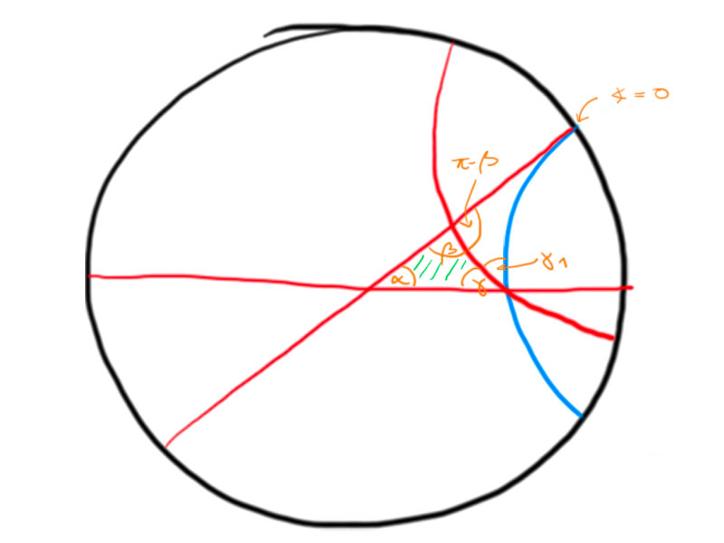
Now,
\begin{align*}
T(\alpha,\beta,\gamma)&=T(\alpha,\gamma+\gamma_1,0)-T(\gamma_1,\pi-\beta,0) \\
&=\pi-\alpha-\gamma-\gamma_1-(\pi-\gamma_1-\pi+\beta)\\
&=\pi-(\alpha+\beta+\gamma)\,.
\end{align*}
Proposition
We can identify the Poincaré and the Klein model by the following construction:
Consider the Klein and Poincaré disc and embed it in $\R^3$ at $x_3=0$ inside the unit sphere (cf. second picture).
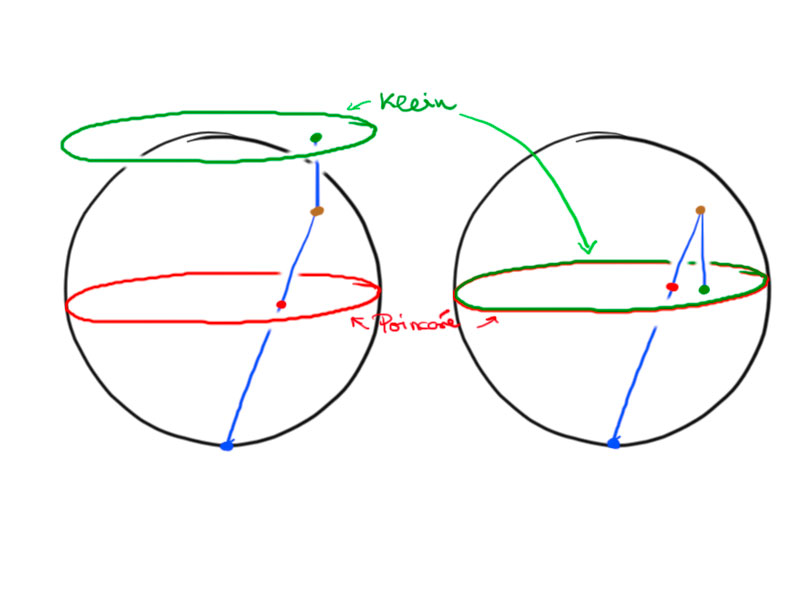
To obtain a point in the Poincaré model from a point in the Klein model, we do the following:
hemisphere back onto the disc.
Corollary
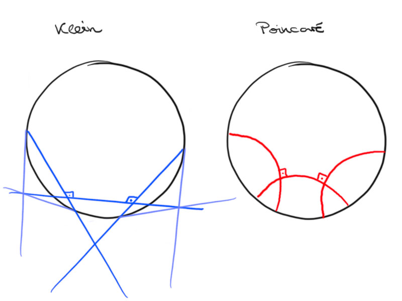
The geodesics in the Poincaré model are circular arcs (or line segments through the origin) that intersect the unit sphere/circle orthogonally.
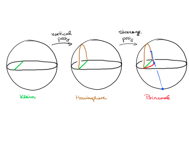
Proof.
In the Klein model geodesics are secants. They are mapped to semicircles that intersect the boundary (the equator) orthogonally in the hemisphere.
Since the steographic projection is conformal and maps circles (or lines) to circles (or lines) the geodesics in the Poincaré disc are circular arcs that intersect the unit circle orthogonally.
Example.
For two lines construct the unique perpendicular.
Remark.
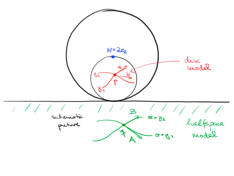
On the way we constructed another conformal model of the hyperbolic space on the hemisphere.
Consider the following map:
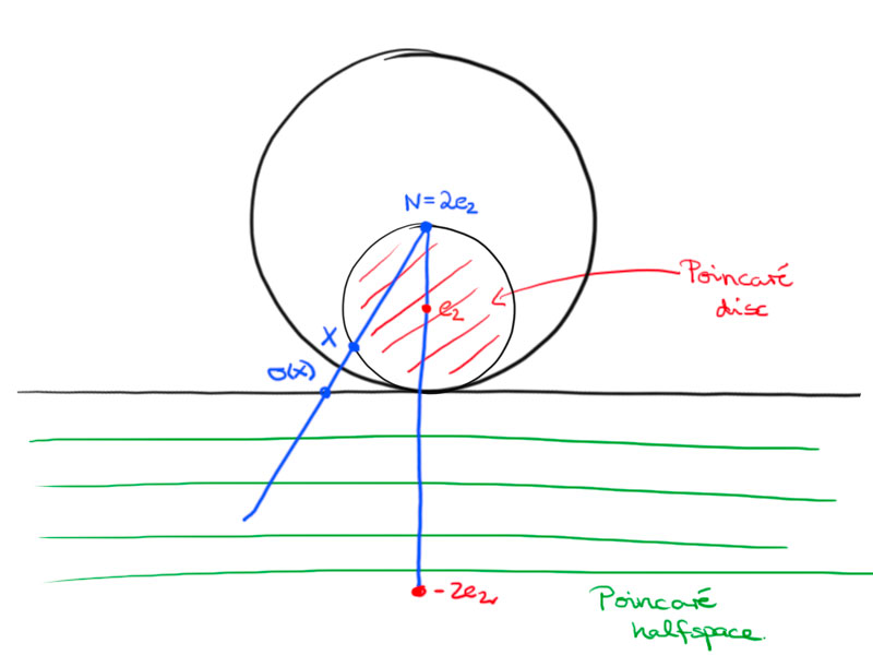
\[\sigma\colon x\mapsto\sigma(x)=2e_2+\frac4{(x-2e_2,x-2e_2)}(x-2e_2)\,.\]
We have $\sigma(S^1+e_2)=(\R\times\{0\})\cup\infty$.
Further, $\sigma(D+e_2)=H_-^2$, where $H_-^2:=\{(x,y)^{\mathrm T}\in\R^2:y<0\}$.
By a similar calculation as the one in the proof of conformality of the Poincaré model we can show the following:
\[(A,B)=\frac{16}{(p-e,p-e)^2)}(a,b)\]
by considering the map
\[\tilde\sigma\colon D\to H_1^2\,,\ p\mapsto2e_2+\frac4{(p-e_2,p-e_2)}(p-e_2)=\sigma(p+e_2)\,.\]
For the hyperbolic metric on the Poincaré model we had
\[g_p(a,b)=\frac4{(1-(p,p))^2}(a,b)=\frac{4(p-e_2,p-e_2)^2}{16(1-(p,p))^2}(A,B)=\frac1{q_2^2}(A,B)\,,\]
where $q=\tilde\sigma(p)$.
Definition
The upper half space $H_+^n:=\{x\in\R^n:x_n>0\}$ endowed with the Riemannian metric
\[g_q(A,B)=\frac1{q_n^2}(A,B)\]
where $q\in H_+^n$ and $A,B$ are tangent vectors to $H_+^n$ at $q$ is the \emph{Poincaré half-space model} of the hyperbolic space.
Properties:
This model is conformal, i.e. the angles between curves correspond to the Euclidean angles.
The geodesics are semi-circles or lines that intersect the boundary orthogonally.
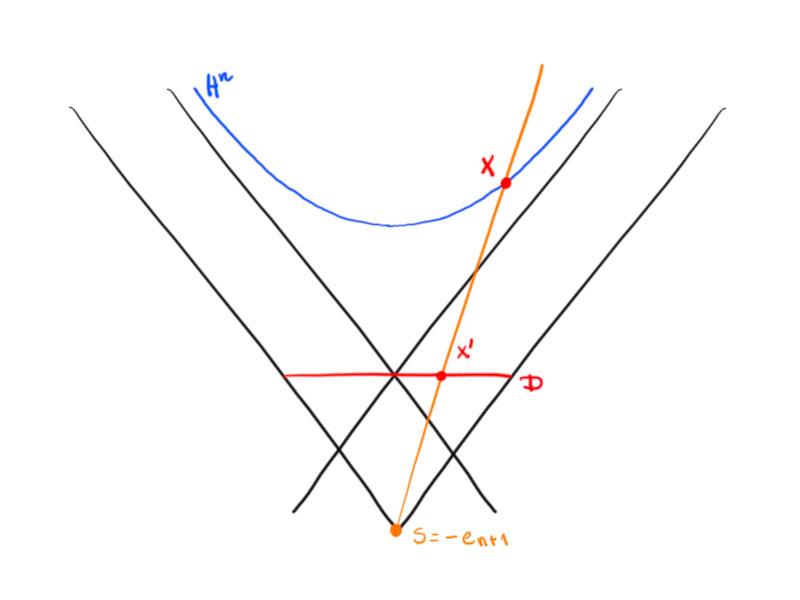
Consider the central projection with center $s$ of $H^n$ onto the plane $x_{n+1}=0$.
This map can be described by
\begin{align*}\sigma\colon H^n
&\to D=\{u\in\R^n:(u,u)<1\}\\
x&\mapsto\frac1{x_{n+1}+1}\begin{pmatrix} x_1\\\vdots\\x_n\end{pmatrix}\,.
\end{align*}
The inverse is given by
\[\sigma^{-1}(u)=\frac1{1-(u,u)}\begin{pmatrix} 2u\\1+(u,u)\end{pmatrix}\,.\]
For $s+t\left(\begin{pmatrix}u\\ 0\end{pmatrix}-s\right)=\begin{pmatrix}tu\\-1+t\end{pmatrix}$ is a point on $\vec{su}$ and
\[-1=\left\langle \begin{pmatrix}tu\\-1+t\end{pmatrix},\begin{pmatrix}tu\\-1+t\end{pmatrix}\right\rangle_{n,1}=t^2(u,u)-(t-1)^2=t^2(u,u)-t^2+2t-1\]
yields $t=0$ or $t(u,u)+2-t=0$ which is equivalent to $t=\frac2{1-(u,u)}$.
This implies $X=\begin{pmatrix}\frac2{1-(u,u)}u\\-1+\frac2{1-(u,u)}\end{pmatrix}=\frac1{1-(u,u)}\begin{pmatrix} 2u\\1+(u,u)\end{pmatrix}$.
The map $\sigma$ is the restriction of the following map to $H^n$:
\[x\mapsto s-\frac2{\langle x-s,x-s\rangle_{n,1}}(x-s)\,,\quad\text{for}\ \langle x-s,x-s\rangle_{n,1}\neq0\,.\]
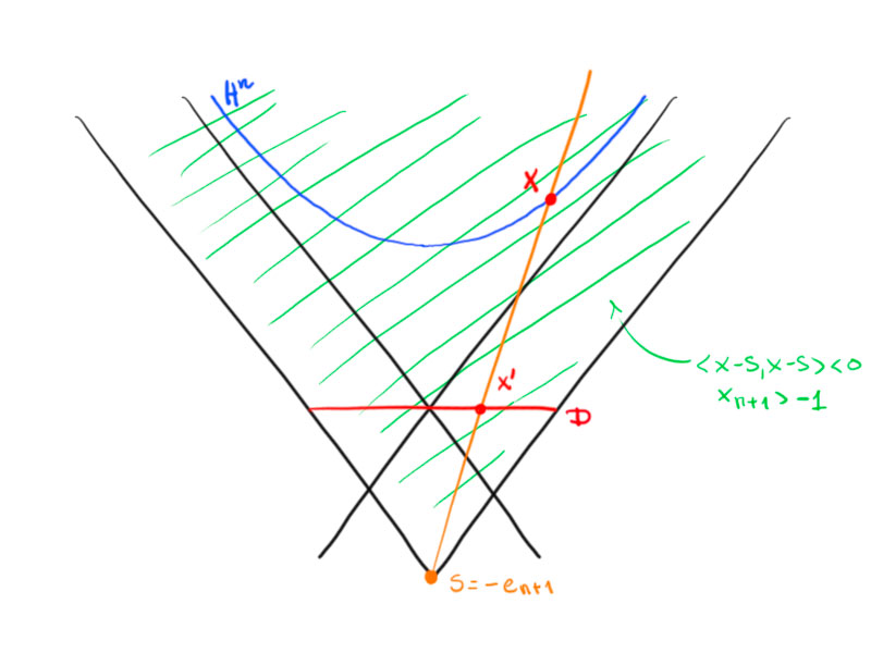
A point $x$ with $\langle x-s,x-s\rangle<0$ is mapped to a point on the ray $\vec{sx}$.
The plane $x_{n+1}=0$ is the orthogonal complement of $s$:
\begin{align*}\left\langle s-\frac2{\langle x-s,x-s\rangle}(x-s),s\right\rangle&=\langle s,s\rangle-\frac{2\langle x-s,s\rangle}{\langle x-s,x-s\rangle}=-1-\frac{2(\langle x,s\rangle-\langle s,s\rangle)}{\langle x,x\rangle-2\langle x,s\rangle+\langle s,s\rangle}\\&=-1-\frac{2(\langle x,s\rangle+1)}{-2-2\langle x,s\rangle}=0\,.\end{align*}
This map is an involution on the set $\{x\in\R^{n,1}:\langle x-s,x-s\rangle-1\}$ with $\sigma(H^n)=D$ and $\sigma(D)=H^n$, where $D\cong D\times\{0\}$.
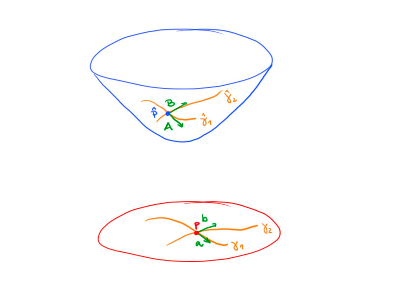
Theorem.
Consider two curves $\gamma_1,\gamma_2\subseteq D$ with $\gamma_1(0)=\gamma_2(0)=p\in D$ and $a:=\gamma_1′(0)$, $b:=\gamma_2′(0)$.
Let $\hat\gamma_1:=\sigma\circ\gamma_1$ and $\hat\gamma_2:=\sigma\circ\gamma_2$ be the corresponding curves in $H^n$ with $\hat\gamma_1(0)=\hat\gamma_2(0)=P=\sigma(p)$ and $A:=\hat\gamma_1′(0)$, $B:=\hat\gamma_2′(0)$.
Then:
\[\langle A,B\rangle_{n,1}=\frac4{(1-(p,p))^2}(a,b)\,.\]
This implies
\[\cosh\alpha=\frac{\langle A,B\rangle}{\sqrt{\langle A,A\rangle\langle B,B\rangle}}=\frac{(a,b)}{\sqrt{(a,a)(b,b)}}\,,\]
where $\alpha$ is the angle of intersection of $\hat\gamma_1$ and $\hat\gamma_2$.
Proof.
Calculate derivatives:
\[A=\hat\gamma_1′(0)=\frac{\mathrm d}{\mathrm dt}\left.\left(s-\frac2{\langle \gamma_1(t)-s,\gamma_1(t)\rangle}(\gamma_1(0)-s)\right)\right\vert{t=0}=-2\frac a{\langle p-s,p-s\rangle}+2\frac{2\langle p-s,a\rangle}{\langle p-s,p-s\rangle^2}(p-s)\,.\]
Similarly,
\[B=-2\frac b{\langle p-s,p-s\rangle}+2\frac{2\langle p-s,b\rangle}{\langle p-s,p-s\rangle^2}(p-s)\,.\]
Now,
\begin{align*}\langle A,B\rangle
&=\frac{4\langle a,b\rangle}{\langle p-s,p-s\rangle^2}-{2\cdot8\frac{\langle p-s,a\rangle\langle p-s,b\rangle}{\langle p-s,p-s\rangle^3}}+{16\frac{\langle p-s,a\rangle\langle p-s,b\rangle\langle p-s,p-s\rangle}{\langle p-s,p-s\rangle^4}}\\&=\frac4{(\langle p,p\rangle-2\langle p,s\rangle+\langle s,s\rangle)^2}(a,b)=\frac4{((p,p)-1)^2}(a,b)\,.\end{align*}
Definition
The open unit ball $D=\{u\in\R^n:(u,u)<1\}$ endowed with the \emph{Riemannian metric}
\[g_u(a,b)=\frac4{(1-(u,u))^2}(a,b)\,,\]
where $a$, $b$ are tangent vectors to $D$ at $u$, is the \emph{Poincaré ball model} of the hyperbolic space.
It is \emph{conformal}, i.e. the hyperbolic angles equal the Euclidean angles.
The \emph{length of a curve $\gamma\colon[0,1]\to D$} is given by
\[\operatorname{length}(\gamma)=\int_0^1\sqrt{g_{\gamma(t)}(\gamma'(t),\gamma'(t))}\mathrm dt\,.\]
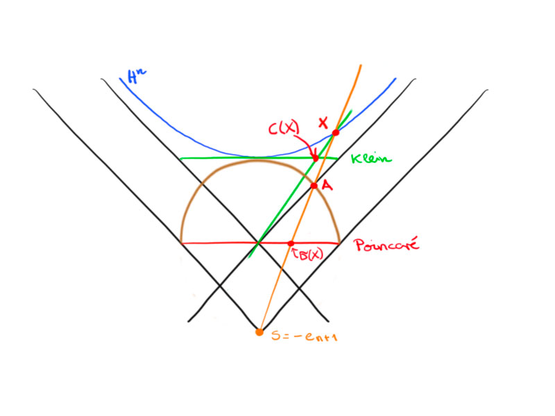
Claim: $A$ is the vertical projection along $e_{n+1}$ of $c(x)$ onto the hemisphere:
\[A_i=c(x)_i\quad\text{for all}\ i=1,\dotsc,n\,.\]
For this, observe that $A=s+t(x-s)$ for some $t$ and $(A,A)=1$.
Thus $\left(s+t\begin{pmatrix} x_1\\\vdots\\x_{n+1}+1\end{pmatrix},s+t\begin{pmatrix} x_1\\\vdots\\x_{n+1}+1\end{pmatrix}\right)=1$ yields
\[1=1+2\left(s,t\begin{pmatrix} x_1\\\vdots\\x_{n+1}+1\end{pmatrix}\right)+t^2\left\lVert\begin{pmatrix} x_1\\\vdots\\x_{n+1}+1\end{pmatrix}\right\rVert^2\]
and hence
\[0=-2t(x_{n+1}+1)+t^2\left(\sum_{i=1}^nx_i^2+x_{n+1}^2+2x_{n+1}+1\right)\,.\]
Now by $\langle x,x\rangle=-1$ we obtain
\[t^2\sum_{i=1}^nx_i^2=t^2(x_{n+1}^2-1)\]
which gives us $t=0$ or
\[t=\frac{2(x_{n+1}+1)}{2x_{n+1}(x_{n+1}+1)}=\frac1{x_{n+1}}\,.\]
So $A=\begin{pmatrix}0\\-1\end{pmatrix}+\frac1{x_{n+1}}\begin{pmatrix} x\\x_{n+1}+1\end{pmatrix}\in\R^{n,1}$.
Thus
\[(A)_{i=1,\dotsc,n}=\frac1{x_{n+1}}x\,.\]
The coordinates of $c(x)$ are given by
\[c(x)=\begin{pmatrix}\frac1{x_{n+1}}x\\1\end{pmatrix}\,.\]
This proves the claim.
Definition.
Let $\ell_1$, $\ell_2$ be two intersecting lines defined by unit normals $n_1$, $n_2$.
The exterior angle $\hat\alpha$ of these two lines is given by
\[\cos\hat\alpha=\langle n_1,n_2\rangle\,.\]
The interior angle $\alpha=\pi-\hat\alpha$ is given by
\[\cos\alpha=-\langle n_1,n_2\rangle\,.\]
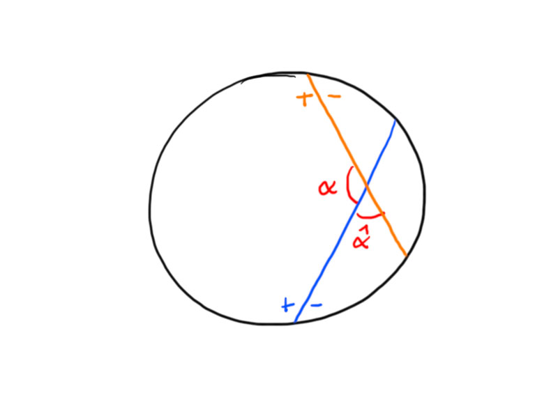
In particular, two lines are perpendicular, if $\langle n_1,n_2\rangle=0$.
Remark.
The Euclidean angle of intersection differs from the hyperbolic angle defined above.
Example
I don’t remember the example 🙁
Proposition
Proof. Homework.
Let $\ell_1,\ell_2\in H^2$ be two hyperbolic lines with unit normal vectors $n_1$, $n_2$:
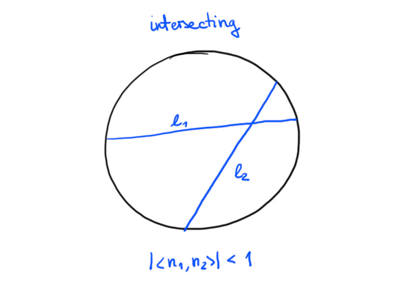
If $\lvert \langle n_1,n_2\rangle\rvert < 1$, then $\ell_1$ and $\ell_2$ intersect.
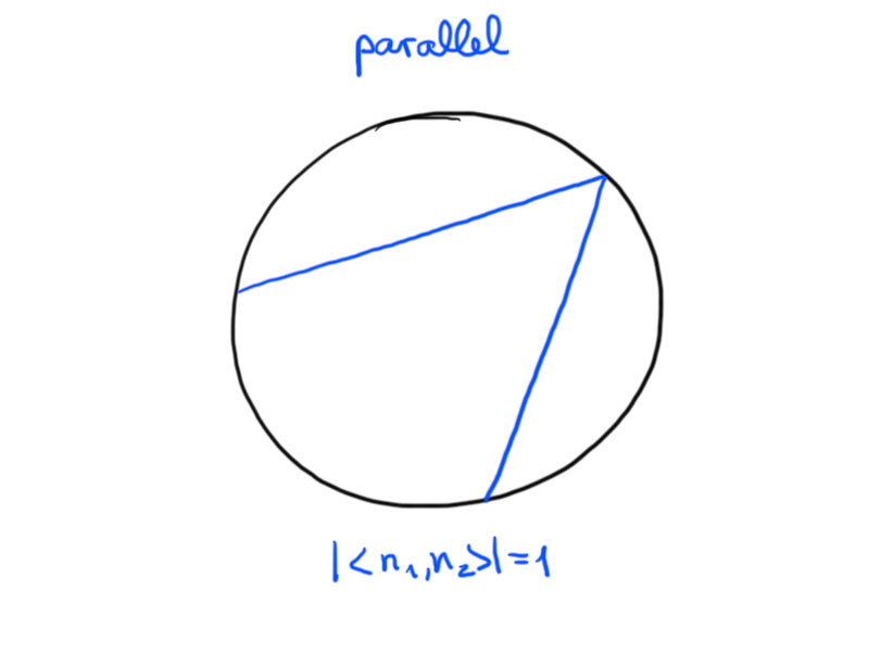
If $\lvert \langle n_1,n_2\rangle\rvert = 1$, we call $\ell_1$ and $\ell_2$ parallel.
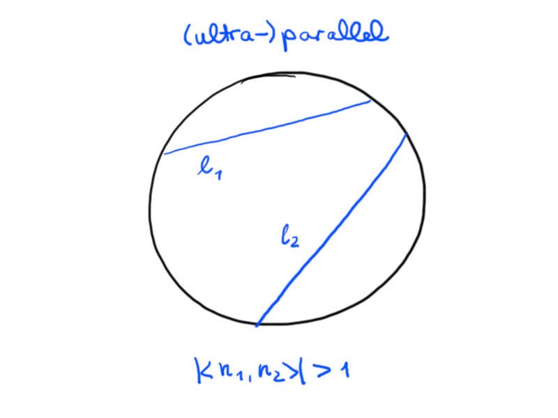
If $\lvert \langle n_1,n_2\rangle\rvert >1$, we call $\ell_1$ and $\ell_2$ (ultra-)parallel.
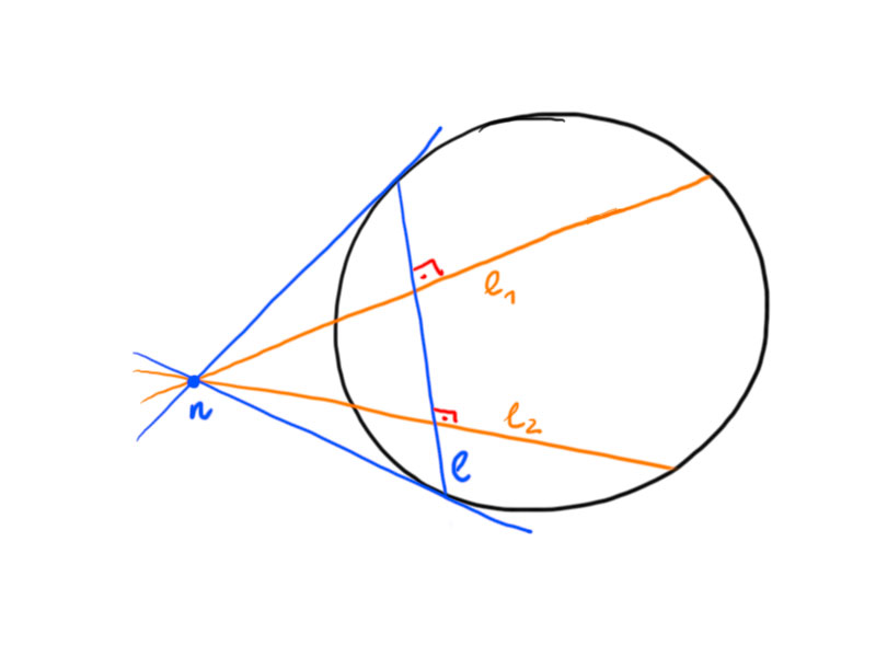
Proposition
The point on a line $\ell\subset H^2$ closest to a point $x\in H^2$ is the intersection point of $\ell$ with its unique perpendicular line through $x$.
Proof.
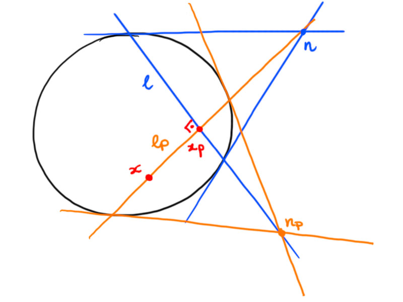
W.l.o.g. assume $x\notin\ell$.
We have
\begin{align*}
\langle n_p,x\rangle&=\langle n_p,x_p\rangle=0&
\langle n,x_p\rangle&=0&
\langle n_p,n\rangle&=0\,.
\end{align*}
We normalize $n_p$ and $x_p$ such that $\langle n_p,n_p\rangle=1$ and $\langle x_p,x_p\rangle=-1$.
Now $\gamma(s)=\cosh(s)x_p+\sinh(s)n_p$ is an arclength parametrization of $\ell$.
The distance from $x$ to $\gamma(s)$ is
\[\cosh d(x,\gamma(s))=-\langle x,\gamma(s)\rangle=-\langle x,\cosh(s)x_p\rangle-\langle x,\sinh(s)n_p\rangle=-\cosh(s)\langle x,x_p\rangle\,.\]
This is minimal for $s=0$, $\gamma(0)=x_p$.
Thus the closest point is $x_p$.
Proposition
Proof.
(i). Consider the arclength parametrization
\[\gamma_p(s)=\cosh(s)x_p+\sinh(s)n\]
of $\ell_p$.
Now
\[x=\gamma_p(s_0)\quad\text{with}\quad s_0=\pm d(x,x_p)\,.\]
Thus
\[\lvert \langle n,x\rangle\rvert =\lvert \langle n,\cosh(s_0)x_p+\sinh(s_0)n\rangle\rvert =\lvert \sinh(s_0)\rvert \,,\]
as $n$ is normalized to $\langle n,n\rangle=1$.
This yields
\[\sinh d(x,\ell)=\sinh d(x,x_p)=\lvert \langle n,x\rangle\rvert \,.\]
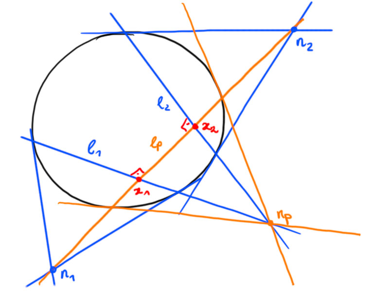
(ii). Parametrize $\ell_1$ as follows:
\[\gamma_1(s)=\cosh(s)x_1+\sinh(s)n_p\,.\]
The distance of $\gamma_1(s)$ to $\ell_2$ is
\[\sinh d(\gamma(s),\ell_2)=\lvert \langle \gamma_1(s),n_2\rangle\rvert =\cosh(s)\lvert \langle x_1,n_2\rangle\rvert \]
since $\langle n_2,n_p\rangle=0$.
This is minimal for $s=0$, i.e. $x_1$ is closest to $\ell_2$ on $\ell_1$
Similarly, $x_2$ is the point closest to $\ell_1$ on $\ell_2$.
Now parametrize $\ell_p$.
\begin{align*}
x_1&=\cosh(s_0)x_2+\sinh(s_0)n_2&
x_2&=\cosh(\tilde s_0)x_1+\sinh(\tilde s_0)n_1\,.
\end{align*}
Here, $s_0=\pm d(x_1,x_2)=\pm\tilde s_0$.
Thus with $\langle n_1,n_1\rangle=1$
\begin{align*}0
&=\langle n,x_1\rangle=\cosh(s_0)\langle n_1,x_2\rangle+\sinh(s_0)\langle n_1,n_2\rangle=\cosh(s_0)\sinh(\tilde s_0)+\sinh(s_0)\langle n_1,n_2\rangle\\
&=\sinh(s_0)(\cosh(s_0)\pm\langle n_1,n_2\rangle)
\end{align*}
and hence $\cosh d(\ell_1,\ell_2)=\lvert \langle n_1,n_2\rangle\rvert $.
Definition.
An affine plane is determined by one equation
\[\langle n,x\rangle_{2,1}=b\]
where $n\in\R^{2,1}$, $n\neq0$, and $b\in\R$.
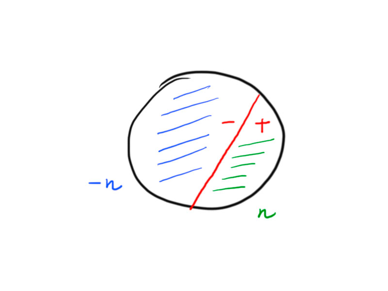
Let $n$ be time-like, $\langle n,n\rangle < 0$.
If $\langle n,n\rangle=-1$, then $n\in H^2$ and $-\langle n,x\rangle=\cosh d(x,n)$ shall be equivalent to $\langle n,x\rangle=b$, i.e. the intersection of the plane given by $\langle n,x\rangle=b$ is a hyperbolic circle around $n$ with radius $r$ such that $\cosh r=-b$ ($b<0$).
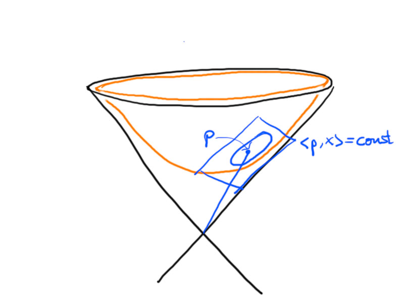
What are the sets defined by space-like and isotropic normal vectors?
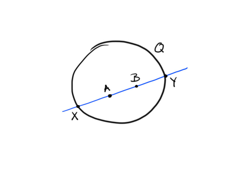
Theorem. For two points $A,B\in H_{\mathrm{pr}}^n$ let $X$, $Y$ be the points of intersection of the line $AB$ with the quadric $Q=\{[x]:\langle x,x\rangle_{n,1}=0\}$, such that $\{A,Y\}$ and $\{B,X\}$ separate each other.
Then
\[d_{\mathrm{pr}}(A,B)=\frac12\log\cr(B,X,A,Y)\,.\]
Proof.
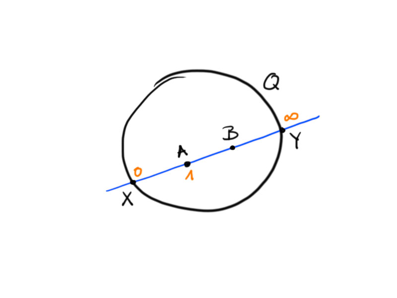
Remember that $\cr(q,1,0,\infty)=q$.
If we choose an affine coordinate such that $X=0$, $A=1$ and $Y=\infty$, then we see that $\cr(B,X,A,Y)>1$, i.e. $\log\cr(B,X,A,Y)>0$.
Parametrize $AB$ by $[a+tb]$ where $A=[a]$ and $B=[b]$.
Solving
\begin{equation}\langle a+tb,a+tb\rangle_{n,1}=0\label{ZeroesForXY}\end{equation}
yields the two solutions $t_1$, $t_2$ such that $X=[a+t_1b]$ and $Y=[a+t_2b]$.
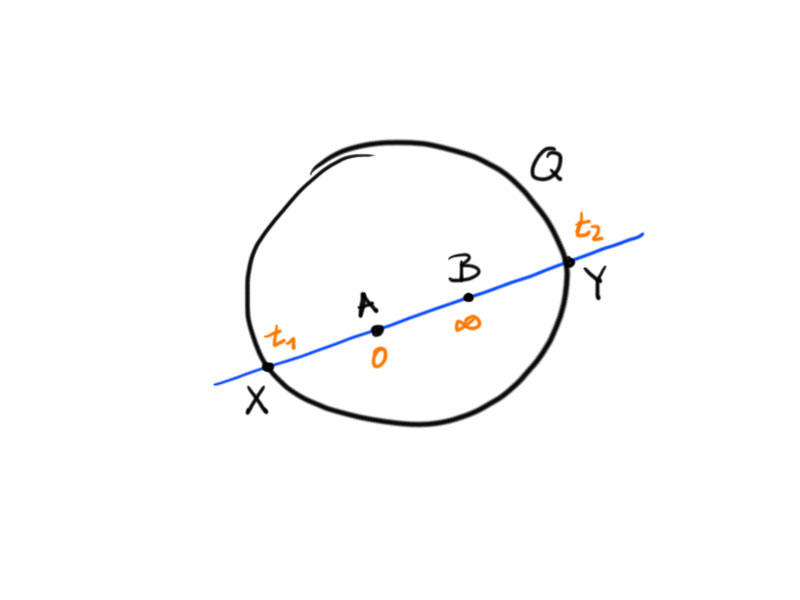
We have $t_1t_2>0$ and: If $t_1,t_2>0$ then $t_2>t_1$, i.e. $\frac{t_2}{t_1}>1$ — if $t_1,t_2<0$ then $t_1>t_2$ and thus again $\frac{t_2}{t_1}>1$.
Looking back at the equation above gives us
\[0=\langle a+tb,a+tb\rangle=\langle b,b\rangle t^2+2t\langle a,b\rangle+\langle a,a\rangle=\langle b,b\rangle(t-t_1)(t-t_2)\,.\]
Comparing the coefficients yields
\begin{align*}
2\langle a,b\rangle&=-\langle b,b\rangle(t_1+t_2)&
\langle a,a\rangle&=\langle b,b\rangle t_1t_2\,,\quad
\text{i.e}\\
t_1+t_2&=-2\frac{\langle a,b\rangle}{\langle b,b\rangle}&
t_1t_2&=\frac{\langle a,a\rangle}{\langle b,b\rangle}\,.
\end{align*}
Thus
\[\cosh d_{\mathrm{pr}}(A,B)=\frac{\lvert\langle a,b\rangle\rvert}{\sqrt{\langle a,a\rangle\langle b,b\rangle}}=\frac{\lvert t_1+t_2\rvert}{2\sqrt{t_1+t_2}}\,.\]
The cross ratio is
\[\cr(B,X,A,Y)=\cr(\infty,t_1,0,t_2)=\frac{\infty-t_1}{t_1-0}\frac{0-t_2}{t_2-\infty}=\frac{t_2}{t_1}\,.\]
This implies
\begin{align*}\cosh\frac12\log\cr(B,X,A,Y)
&=\frac12\left(\mathrm e^{\frac12\log\frac{t_2}{t_1}}+\mathrm e^{-\frac12\log\frac{t_2}{t_1}}\right)=\frac12\left(\sqrt{\frac{t_2}{t_1}}+\sqrt{\frac{t_1}{t_2}}\right)\\
&=\frac12\frac{\lvert t_2\rvert+\lvert t_1\rvert}{\sqrt{t_1t_2}}=\frac12\frac{\lvert t_1+t_2\rvert}{\sqrt{t_1t_2}}\,,
\end{align*}
since $t_1t_2>0$.
Hyperbolic lines are secants of the unit ball
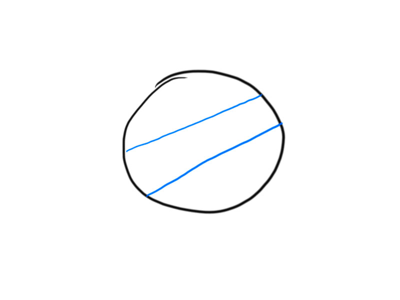
Obviously, to a line and a point in $H^2$ there exist many lines through the point that do not intersect the line:
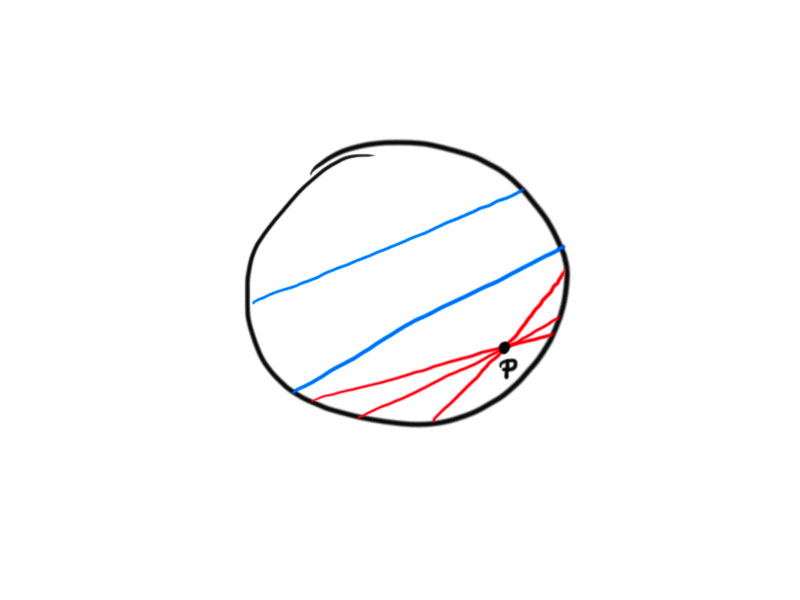
This contradicts the Parallel Axiom.
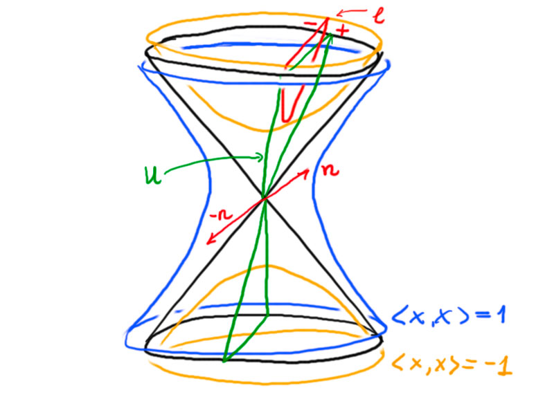
Using polarity, we can assign unit normal vectors to hyperbolic lines in $H^2$.
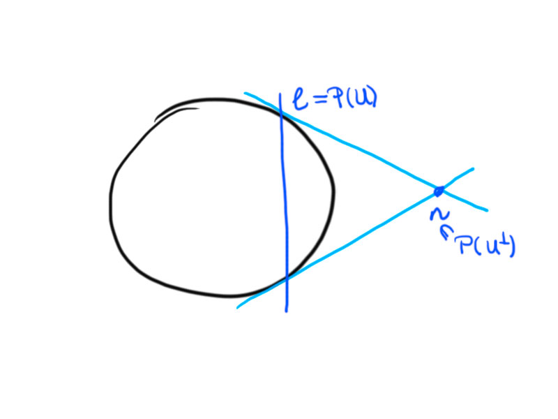
With $\ell=P(U)$, where $U$ is a two-dimensional subspace with signature $(+-)$ (where by the signature of a subspace $V$ we denote the signature of $\langle\cdot\,,\cdot\rangle$ restricted to $V$) we have $n\in P(U^\perp)$, where $U^\perp$ has signature $(+)$ – so we can choose $n$ with $\langle n,n\rangle=1$.
For every line there exist two unit normal vectors defined via polarity with respect to $\langle\cdot\,,\cdot\rangle_{n,1}$.
There is a bijection between half planes and vectors $n\in\R^{2,1}$ with $\langle n,n\rangle=1$.
Proposition
Let $\ell_1,\ell_2\in H^2$ be two distinct lines in the hyperbolic plane with unit normals $n_1$, $n_2$ (i.e. $\langle n_1,n_1\rangle=1$ and $\langle n_1,p\rangle=0$ for all $p\in\ell_1$).
Then the following are equivalent:
- The two lines intersect.
- $\operatorname{span}(n_1,n_2)$ has signature $(++)$.
- $\lvert\langle n_1,n_2\rangle_{2,1}\rvert<1$.
Proof
(i)$\Rightarrow$(ii): Let $\ell_1\cap\ell_2=:x$.
Then $\operatorname{span}\{x\}$ has signature $(-)$, since $\langle x,x\rangle=-1$.
Thus $\operatorname{span}\{x\}^\perp$ has signature $(++)$ and $n_1,n_2\in\operatorname{span}\{x\}^\perp$.
This implies $\operatorname{span}\{n_1,n_2\}=\operatorname{span}\{x\}^\perp$ has signature $(++)$.
(ii)$\Rightarrow$(i) can be shown similarly.
(ii)$\Leftrightarrow$(iii):
The matrix for $\langle\cdot\,,\cdot\rangle\big\vert_{\operatorname{span}\{n_1,n_2\}}$ is given by
\[A=\begin{pmatrix}\langle n_1,n_1\rangle&\langle n_1,n_2\rangle\\\langle n_1,n_2\rangle&\langle n_2,n_2\rangle\end{pmatrix}=\begin{pmatrix}1&\langle n_1,n_2\rangle\\\&1\end{pmatrix}\,.\]
$A$ is positive definite if and only if $\operatorname{span}\{n_1,n_2\}$ is $(++)$, which is (ii).
But also, positive definiteness if equivalent to $1>0$ and $1-\langle n_1,n_2\rangle^2>0$, which is (iii).