Ames Room update. At the beginning of the lecture Mr. Dr. Gunn returned to exercises he gave in class last week.  He showed that the projective matrix for the simplified 2D Ames room looks like: \[ \left( \begin{array}{ccc} 1 & 0 & 0 \\ 0 & 1 &0 \\ \dfrac{1}{n} & 0 & 1 \end{array} \right)\] where $n$ is the distance in meters to the right of the eye point, which is the image of the ideal point in the x-direction.  As a result, Dr. Gunn asserted (shamelessly without proof) that any projectivity can be decomposed as the product of an affine matrix and an “Ames” projectivity — the latter being defined as a matrix, like the one above,  which is the identity matrix except in the last row.

Geometry Factories This week we turned to discussing how geometry is represented in jReality. The basic classes PointSet, IndexedLineSet, and IndexedFaceSet were introduced.  However, using these classes directly is awkward and time-consuming.  Instead, there is a set of geometry factories which do the heavy lifting and allow the user to specify the geometry in a more mathematical way.  We concentrate on the factory ParametricSurfaceFactory. This allows the user to specify an immersion of a rectangular domain in $\mathbb{R}^2$ into $\mathbb{R}^3$ or $\mathbf{P}^3$ (depending on whether one uses standard or homogeneous coordinates).

Assignment3 This assignment is designed to provide some practice in using geometry factories.  In contrast to Assignment2, where you were asked to create a scene using very simple geometry and many transformations, in this assignment you are forbidden (Verboten!) to use matrices to “create” geometry, you have to use … geometry!  Check out the latest version from the teacher git repository (the Tuesday tutorial participants have already made this step.)  However, note that even if you were at the Tuesday tutorial, you should still update again since I’ve cleaned up the assignment and focused it more on the actual task at hand — I’ve removed the torus for example and have used the time parameter to rotate the square around — which is forbidden but it’s useful to see how a simple example works.

Update to Assignment3 [15.11].  I’ve updated Assignment3Example based on an example worked out in yesterday’s tutorial, which in turn was suggested in the classroom discussion yesterday.  The result is that the example now rolls up the square into a cylinder: 

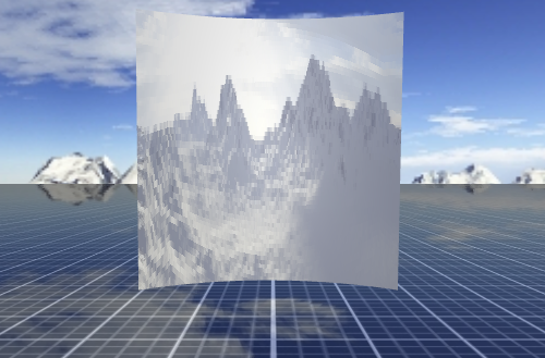
How it’s done: The first step is to set two fields in the setValueAtTime() method: the time and the radius of the cylinder r.  The radius depends on the time in such a way that it interpolates between $\infty$ and $\dfrac{1}{\pi}$ as $t$ varies between 0 and 1:

@Override
public void setValueAtTime(double d) {
        time = d;
	r = (time == 0) ? -1 : 1/(Math.PI*time);
	surface.update();
}

Then when the factory is updated, the evaluate() method uses these fields to construct a section of a vertical cylinder with radius $r=\dfrac{1}{\pi}$. The time $t=0$ is handled separately to produce the beginning square. The displayed section of this cylinder is subject to two constraints:

1. It subtends a horizontal arc length of 2 (to be consistent with the fact that the beginning square has side length 2), and
2. The vertical mid-line of the square remains fixed in space throughout the animation.

Condition 1) implies that the section of the cylinder subtends an angle of $t\pi$ so that it has arc length 2 as desired.  Furthermore we choose the $(u,v)$ domain so that it goes from $(-1,-1)$ to $(1,1)$  and the values of $u=0$ corresponding to the vertical mid-line of the square are fixed: the square rolls up while keeping this line fixed.  In order for this line to be fixed, we calculate that the axis of the cylinder has to have $xyz$ coordinates $(0, y, r)$.  Taken together, this produces the following code for $evaluate()$:

@Override
public void evaluate(double u, double v, double[] xyz, int index) {
	double angle = time * u * Math.PI;
	xyz[0] = time == 0 ? u : r * Math.sin(angle);
	xyz[1] =  v;
	xyz[2] = time == 0 ? 0 : -r * Math.cos(angle) + r;
	xyz[3] = 1.0;
}

To satisfy the assignment, this animation would need to be continued so that at the end $t=1$ the cylinder has unrolled again so that the opposite side faces out.

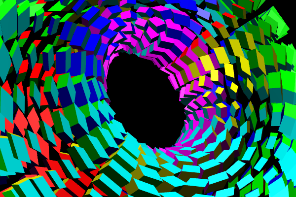
3D Video Transitions: Practical applications of Assignment3. Due to some very important work I’m doing this week for Matheon, I’m not able to write such detailed blog posts as usual.  This movie is a “cross-eyed stereo” movie meaning if you can cross your eyes just the right amount as you watch it, the images should fuse together to produce 3D depth.  If you do view this movie, you’ll see that it consists of 3D transitions between still photos — the kind of transition I mentioned in class when I introduced Assignment3! So everything hangs together.  In any case, everything you need to know to do Assignment 3 should be contained in the Java classes from the git repository.  If not let me know. The assignment is due on Friday November 22, which is, if I’m not mistaken, the 50th anniversary of the assassination of John F. Kennedy, an event which I experienced as a 6th grader.

Assignment2 Update [11.11.2013] I’ve added some points to the discussion of Assignment2, to include how to get the inspector properly configured, and how to store and restore properties.  Please take a look at these additions and extend your own code if you need to.

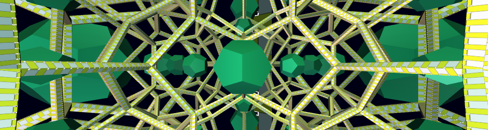
•  I’m continuing to enjoy looking at the results of Assignment2.  The assignments I’ve looked at look good. I’ve particularly enjoyed the ones with which have implemented the torus setup.  Following picture shows a frame from the animation based on a torus.  It reminds me of “op art”. They are recognizably cubes, but each looks like it was  drawn using a different perspective.
• I’ve added a bit more functionality to Assignment2, so you can play around with the tool in the leaf child, that I demo-ed last Thursday 07.11.13 in class. (Exercise: why is 07.11.13 a special day. Hint: it has to do with prime numbers.).  It’s designed so that if you update your repository to my gitorious repository (the one we named “teacher”) your code should continue to function unchanged, but the inspector now contains a button which allows you to activate a translate tool in the leaf component.  If however you construct your own inspector w/o using a call to super.getInspector(), this button won’t appear for you.

Projects: It’s still early in the process for choosing a project.  You may be interested in these guidelines from last year.

Teamwork:  You are expected to work in teams.  It’s more fun and the results are of higher quality (IMHO). We can discuss any technical problems with team building today.

05.11 Lecture: Dr. Gunn took the opportunity to present an introduction to the jReality scene graph.   Look also here for a more sober introduction to the same topic. As Assignment2 (below) is easy, you are encouraged to spend some time in the next week familiarizing yourself with the jReality developer tutorial, particularly the sections devoted to transformations, geometry, and appearances. You can do this using your browser and webstart, but if you want to play with the code for particular examples (strongly recommended), these reside in the jReality project under the src-tutorial folder.

07.11 Lecture: We looked in more detail at the SceneGraphComponent javadoc. We also looked at the base class SceneGraphNode and its subclasses. Then, departing from his original plan to discuss the  Appearance class,  Dr. Gunn turned the discussion to the tool system, and showed how to add a tool to the leaf child of Assignment2 in such a way that the resulting transformation was applied before the animation transformation (coming from setValueAtTime()), with interesting results. This discussion also hopefully established the importance of the SceneGraphPath class in determining the exact position of a node in the scene graph.

Assignment1 is completed and the results are, from my point of view, very satisfactory.  To begin with, most of the technical difficulties have been overcome and I have “harvested” git repositories for the majority of the students who have signed up for the class.  And secondly, the quality and variety of the turned-in assignments is impressive.  I only wish it were easier to collect all the different assignments into a “composite” application to be shared and enjoyed by all.  If anyone has any ideas how this can be technically achieved please get in touch with me.  Otherwise I will continue to show a few samples during the tutorial sessions as time permits.

Assignment2 is already there, due this Friday at midnight. It’s basically Assignment1 the way it should have been.  Includes storing and saving properties,  on-line documentation file, and a more modular structure.  Just take what you did for Assignment1 and convert it to the improved format.  Of course if you want to improve it (for example with the extra credit idea), please do so.  In particular, here are the directions:

• Follow the directions here to update the course repository.  You should find a new package template.assignment2.  To prepare your own version of assignment2, do the following, assuming your package name is student007:
  • Create a package student007.assignment and copy into it the files assignment2.xml, assg2-anim.xml, Assignment2.html, and assg2-01.png.
  • In this package create a new Java class named Assignment2.  It should inherit from the class template.assignment2.Assignment2.
  • Edit the newly created class.  You should see stubs for the following methods, which are declared abstract in the superclass:
    • protected Matrix getSetupMatrix(int i, int j)
    • protected Matrix setArrayValueAtTime(double time, int i, int j)
    • protected String getPropertiesFile()
    • protected String getDocumentationFile()
  • If you look into template.Assignment2 or template.Assignment you can see how these methods should be used.
  • Copy code from your original Assignment1 into these method stubs to create a running application that does the same thing your original assignment1 did.  getPropertiesFile() should return “src/student007/assignment2/assignment2.xml” and getDocumentationFile() should return “Assignment2.html”.
  • If you’ve added a slider to the inspector (which was part of the assignment), you’ll also need to override the getInspector() method.  To add your GUI elements, you can call super.getInspector(), cast the return value to an instance of Box, and add your GUI elements to this box.  Or don’t call super.getInspector(), and construct the complete inspector in your method.
  • On a related note, if you’ve added parameters which you want to store and restore as properties, you’ll need to overwrite storeState() and restoreState() (look into the parent class to see how this is done).
  • Run the program.
    • Verify that the on-line documentation works by typing the ‘h’ key — your browser should open a window and display the provided html file.  Edit it to reflect what your group did. You can use a normal text editor to do this if you don’t have access to an html editor — just ignore all the html formatting and replace the text sections with text that describes your application.
    • Also verify that the properties file and animation file are working by changing some parameters and saving them (save the property file by choosing File->Quit, save the animation file by choosing “File->Save As…” and saving it in student007/assignment2/assg2-anim.xml.)
  • Notice that the parameters in the left inspection panel are now saved in the properties file.  If you have other parameters or have removed some of these, please overwrite the methods storeStates() and restoreStates() (see template.assignment2.Assignment2 for details).
  • Note that the inspector panel of the Assignment2 superclass contains the 5 parameters provided by the template assignment.  If you still use these but have added more of your own, you can implement the method getInspector(), and add your new GUI elements to the component which super.getInspector() returns.  (You may have to cast this to class Box to be able to add components to it.)

• Extra credit assignment. There is now a method Pn.projectivity(double[] dst, double[][] from, double[][] to) which provides the projective matrix mapping the $n+2$ points from onto the $n+2$ points to.  Of course to get it you’ll need to update your jreality repository which we’ll do in the tutorial this week, or see the post describing the steps.

Show working version of movie on conformal maps.

The lecture on 22.10 began with a repetition of the “guided visualization” from the first meeting on 15.10.  Then Dr. Gunn demo-ed a couple of dynamic geometry applets demonstrating two theorems from the “early days” of projective geometry (circa 1640): Desargues Theorem and Pascal’s Theorem, emphasizing the qualities of mobility and variety which both theorems exhibit. Links can be found on the previous post.

Coordinates for projective geometry. When projective geometry was rediscovered in the 1820’s, the mathematics was available to introduce coordinates.  In modern form, this can be expressed as the projectivization of $\mathbb{R}^n$ introduced in the previous lecture:   \[\mathbf{P}^2(\mathbb{R}) := \mathbb{R}^3~/~\sim \text{  where } \mathbf{P} \sim \mathbf{Q} \iff \mathbf{P} = \lambda \mathbf{Q} \text{ for } \lambda \neq 0\].

Note: the following discussion focuses on the case of the projective plane $\mathbf{P}^2(\mathbb{R})$.  Everything said here generalizes easily to general dimension $n$, in particular to $n=3$ which is the case we are really interested in.

Projective transformations and the projective group.  A projective transformation, or projectivity for short, is defined as an invertible self-map of $\mathbf{P}^n(\mathbb{R})$ which preserves lines.  Here, a line is the set of points spanned by two points: $\alpha \mathbf{P} + \beta \mathbf{Q}$ for $\alpha, \beta \in \mathbb{R}$.  It’s not hard to see that this corresponds to a plane through the origin in $\mathbb{R}^{n+1}$.   An invertible self-map of $\mathbb{R}^{n+1}$ which maps planes to planes is what is called a linear map, and satisfies $f(\alpha \mathbf{P} + \beta \mathbf{Q}) = \alpha f(\mathbf{P})+\beta f(\mathbf{Q})$.  The set of all such self-maps forms a group, called the general linear group of dimension $n+1$, and written $GL(n, \mathbb{R})$.  Once a basis has been chosen one has a representation as matrices, hence $GL(n+1,\mathbb{R})$ is sometimes called a matrix group.

Exercise: Show that an element of $GL(n+1,\mathbb{R})$ induces a self-map of $\mathbf{P}^n(\mathbb{R})$ which maps lines to lines, that is, is projective.  And conversely, a projective transformation comes from some element of  $GL(n+1,\mathbb{R})$.  Two matrices give rise to the same projective transformation $\iff$ they are non-zero multiples of each other.

Hence the group of projectivities is the quotient of $GL(n+1)/ \mathbb{R}$.  It is written $PGL(n+1,\mathbb{R})$ to indicate that it results from projectivizing $GL(n+1,\mathbb{R})$. It has one less dimension than $GL(n+1)/ \mathbb{R}$.  Hence $PGL(3,\mathbb{R})$ has dimension $9-1=8$.

The group $$PGL(n+1,\mathbb{R})$ includes a huge range of possible transformations. A basic result which characterizes this group is:  a projectivity is uniquely determined by  choosing any $n+2$ points to be mapped to any other $n+2$ points (of course the points must be in general position).  The study of possible projective transformations is an interesting subject in its own right but one which we have to pass by right now.

Often one is interested only in the affine subgroup, that is, the transformations that map the ideal elements to themselves.  Exercise:  An affine transformation has last row $(0,0, ….,0,1$).

Among the affine transformations, one is interested particularly in isotropic scaling by the factor $\lambda$.  Such a transformation has a diagonal matrix all of whose diagonal entries are $\lambda \neq 0$, except the last one which is, as noted, 1.  For this course we will be particularly interested in the subgoup of the affine group that preserves distance and angle:

Euclidean Isometries. Recall that a euclidean transformation is a self-map of euclidean space that preserves euclidean distances and angles.   Exercise: A euclidean isometry is a projectivity.    Hence we can identify the euclidean group with a subgroup of $PGL(n+1, \mathbb{R})$.  Furthermore, the set of orientation-preserving isometries $\mathbf{E}^+(n)$ is a subgroup of the full euclidean group $\mathbf{E}(n)$.  Exercise: An isometry is orientation-preserving $\iff$ its determinant is positive.

Exercises.  All these exercises refer to the euclidean plane.

1. A euclidean translation by the vector $\mathbf{u} = (x_u, y_u)$ is given by the matrix\[ \mathbf{T}_{\mathbf{u}} = \left( \begin{array}{ccc} 1 & 0 & x_u \\ 0 & 1 & y_u \\ 0 & 0 & 1 \end{array} \right)\]
2. A euclidean rotation around the origin by angle $\alpha$ is given by the matrix \[ \mathbf{R}_{O,\alpha}  =  \left ( \begin{array}{ccc} \cos{\alpha} & -\sin{\alpha} & 0 \\ \sin{\alpha} & \cos{\alpha}  & 0 \\ 0 & 0 & 1 \end{array} \right)\]
3. Write the matrix form for a rotation $\mathbf{R}_{\mathbf{C},\alpha}$around the point $\mathbf{C} = (x_c, y_c)$ through angle $\alpha$.  [Hint: $\mathbf{R}_{\mathbf{C},\alpha} = \mathbf{T}_{\mathbf{C}} \circ \mathbf{R}_{O,\alpha} \circ \mathbf{T}_{\mathbf{-C}}$.]

How translations and really a kind of rotation [optional].  One of the unusual aspects of euclidean geometry is that translations and rotations seem so different, yet both are isometries.  Using the projective model we have developed, it’s possible to argue that a translation is really a kind of rotation.  Consider the translation $\mathbf{T}_{(1,0)}$ with translation vector $(1,0)$.  Imagine the series of rotations $R_n$ indexed by $n$ with center $(0,n)$ through an angle $\dfrac{1}{2 \pi n}$. Exercise: For any bounded region $D$ of the plane, I can find an $n_0$ such that $R_n -\mathbf{T}_{(1,0)}$ for $n> n_0$ is arbitrarily small for any point in $D$.  Taking this to the limit, one arrives at the conclusion that the translation $\mathbf{T}_{(1,0)}$ can be thought of as a rotation around the ideal point $(0,1,0)$ through a distance (not angle!) 1. Similar results apply for any translation; the “center point” is then the ideal point in the direction perpendicular to the translation.

Conclusion. This concludes the theoretical introduction to how euclidean isometries can be expressed as matrices. The next step is to study the jReality classes:

1. de.jreality.math.Rn  This class provides general report for the euclidean vector space $\mathbb{R}^n$.  This includes multiplying matrices times vectors and other operations from linear algebra.
2. de.jreality.math.MatrixBuilder  This is the primary class for constructing euclidean isometries.

Equipped with this knowledge, you should then be prepared to go to work on Assignment1.  For details consult the Javadoc for the Java class in eclipse.

The Renaissance was a time of great innovation in all areas of European life.  Science, art, and religion all received powerful new impulses.  I focused on the development of painting, where the invention of perspective painting had important consequences for mathematics. The first perspective paintings appeared around 1420 (Masaccio).  The slides containing the paintings discussed in the lecture can be found here.

From Art to Geometry. Around 100 years later the process had been mechanized (Dürer), and finally, after another 100 years, the French architect and mathematician Rene Desargues published a book (1642) which provided a new geometry to represent perspective painting.  This new geometry is called projective geometry.  The name comes directly from its roots in perspective painting, as follows.

Central Projection. The essential operation of perspective painting was identified as a central projection, in which points in the world are projected onto points of an image plane by means of lines passing through the center point of the projection (think of the eye of the painter, and the image plane as a plane standing between the painter and the world — which he transfers to his canvas). The essential problem in terms of describing such a projection geometrically was the existence of vanishing points: points in the image where parallel lines in the world appear to meet.  It was awkward to have a pairing of points in which some points did not have a partner: the vanishing points on the image had no real partner point in the world since parallel lines, by definition, do not meet.

Ideal elements. Desargues innovation was to suppose that parallel lines in fact do meet, in a special sort of point, an ideal point.  All lines parallel to a given line share the same ideal point. All the ideal points of all the lines in a plane go together to form a line, the ideal line of the plane. (You might think they would form a circle, but since it’s “infinitely” far away, it can’t be curved, so is a line.)  And all the ideal points of all the lines in space form a plane, the ideal plane.  (These ideal points bear a strong resemblance to free vectors, see Exercise 3 below.)

The first flower. Desargues developed his new geometry, based on the addition of these ideal elements to the ordinary elements, purely synthetically, that is, without coordinates. He discovered beautiful theorems (for example, Desargues Theorem).  His younger colleague, Blaise Pascal, contributed other remarkable theorems, such as Pascal’s Theorem. But the new geometry was too far ahead of its time.  The geometry of Desargues’ friend Rene Descartes was better suited to  new impulses in natural science which remained within the framework of euclidean geometry.  Cartesian geometry spread rapidly, while Desargues’ work was forgotten and disappeared.  It was rediscovered, independently, in 1822 by another Frenchman, Jean-Victor Poncelet, and has since then developed into a broad and deep branch of mathematics.  There is reason to believe that it may yet prove useful to the further development of natural science just as Cartesian geometry has been useful during the past 400 years.

When it was rediscovered, projective geometry was outfitted with coordinates, it is these coordinates which I want now to describe, since they are important to the field of mathematical visualization.

Mathematical definitions. The real projective plane $\mathbf{P}^2(\mathbb{R})$ is defined by applying an equivalence relation to the euclidean vector space $\mathbb{R}^3$.  Two points with coordinates $(x,y,z)$ and $(x’,y’,z’)$ are defined to be equivalent $\iff$ $(x’,y’,z’)=(\lambda x, \lambda y, \lambda z)$ for some $\lambda \neq 0$.  This equivalence relation can be expressed geometrically by saying, “the points of the projective plane are the lines of $\mathbb{R}^3$}”.   Each projective points has many possible representatives $(\lambda x, \lambda y, \lambda z)$ from $\mathbb{R}^3$.  We write $(x,y,z)$ (a bit sloppily) to mean the equivalence class of $(x,y,z)$.

The connection to Desargues. In this definition of the projective plane, where are the “ordinary” points and where are the “ideal” points discussed above?  The simplest answer is to define a point $(x,y,z)$ to be ordinary if $z \neq 0$, and to be ideal if $z = 0$.  In the former case, we can choose $\lambda = \dfrac{1}{z}$ to obtain an equivalent representative point $(\dfrac{x}{z}, \dfrac{y}{z}, 1)$.  Hence we can assume the ordinary points are of the form $(x,y.1)$ while, as we show below, the ideal points appear in the form $(x,y,0)$.  We call these coordinates affine coordinates for the projective plane.

Intersection of parallel lines. Let’s apply this framework to the problem of representing the intersection of parallel lines.  If we represent a line by its line equation in ordinary coordinates, it has the form $ax+by+c=0$ where not both $a$ and $b$ are zero.  Using affine coordinates, this takes the form $ax+by+cz=0$.  In this form the expression is symmetric in $(a,b,c)$ and $(x,y,z)$ hence $(x,y,z)$ coordinates for the projective plane are sometimes called homogeneous coordinates. It’s clear that if $(x,y,z)$ satisfies the line equation, then so does $(\lambda x, \lambda y, \lambda z)$ for $\lambda \neq 0$, hence the line equation is well-defined for points of the projective plane, and our choice of $z=1$ is not essential.

Exercises

1. Intersection of two lines.
   1. Show that the intersection of the two lines $l : ax+by+cz=0$ and $m : dx+ey+fz=0$ is the projective point $(bf-ce, -af+cd, ae-bd)$. [Hint: show this expression satisfies both equations.]
   2. Show that $l$ and $m$ are parallel $\iff$ $ae-bc = 0$, hence the intersection point $(x_i, y_i, z_i)$ is ideal $\iff$ $z_i = 0$. Hence the ideal line of the plane is given by the equation $z = 0$.
   3. The ideal point of the line with equation $ax+by+cz=0$ is $(b, -a, 0)$. [Hint: apply A + B above.] Conclude that all lines of the form $ax+by+cz=0$ for fixed $a$ and $b$ have the same ideal point $(b,-a,0)$.
2. Joining line of two points.
   1. Show that the joining line of  two points $P : (x_0,y_0,z_0)$ and $Q: (x_1,y_1,z_1)$  is the line with line equation $ax + by + cz = 0$ where $(a,b,c) = (y_0 z_1 – y_1 z_0, x_1z_0 – x_0 z_1, x_0 y_1 – x_1 y_0)$. [Hint: show that both points satisfy this equation.]
   2. In high school, using traditional Cartesian coordinates, perhaps you learned that the line through the point $P := (x_0,y_0)$ with direction vector $V := (u,v)$ has line equation $-vx +uy + x_0v-uy_0 = 0$.  Show that you obtain the same line equation in the projective setting by joining the point $(x,y,1)$ with the ideal point $(u,v,0)$ using the formula in part A above.
   3. Result B) above implies that a free vector in Cartesian geometry is similar to an ideal point in projective geometry.  Consider other properties of free vectors and test whether and how they carry over to ideal points.  For example, a vector is often defined as the difference of two points.  (For this exercise, assume that we are using affine coordinates for the ordinary points in $\mathbf{P}^2(\mathbb{R})$, i.e., points have the form $(x,y,1)$.)  On the basis of this, discuss the following statement:  “An ideal point is a direction.”

Hopefully these exercises have convinced you that projective geometry in fact solves the problem posed by vanishing points, and provides a  representation with which we can compute practical problems.

Eye and hand:   There are in good reasons to deny the existence of the ideal points of projective geometry, as well as to assert their existence.  How can one resolve this contradiction? One way is to understand the two positions as representing two different human sense organs.  The euclidean view, that parallel lines do not meet,  is derived from the evidence provided by the sense of touch.  I can never hope to touch an ideal point since if I try to move towards it, the parallel lines remain the same distance apart.  On the other hand, the sense of sight sees the parallel sides of a train track intersect at the horizon as clearly as the sense of touch knows they stay the same distance apart forever.  The different senses give rise to different geometries.  Neither one is right or wrong, just different.

Exercise. It’s only been around 600 years, since the early Renaissance, that human beings (first just a few, now everyone) have been conscious of seeing parallel lines intersect in a “realistic” perspective picture. Why do you think this development took so long to occur?

Resources: For more detailed treatments of projective geometry see the resources listed on the webpage for the course Geometrie I, such as these lecture notes by Boris Springborn.

Coming next: Using projective geometry to represent geometric transformations, such as translations, rotations, scaling, and more.

We start out on our expedition.  We began by doing some “guided mathematical visualization” with our eyes closed, led by Dr. Gunn.  At the other extreme Dr. Gunn asked whether a crystal he brought with him represents “mathematical visualization”. We chose to leave unanswered the question of whether some being could have thought the crystal into existence as a kind of “mathematical visualization”.  In any case we decided that neither example qualified as a mathematical visualization (MV) in the sense of this course.  To be a MV in the sense of this course means to combine something of the thought quality of pure mathematics with the sense-perceptible, material nature of the crystal.  It must be an “embodiment” of mathematics.

Next, Dr. Gunn introduced 3 types of “product” that qualify as mathematical visualization:

1. 3D prints (the ones he passed around he had made in the last 6 years at the 3D Lab at TU Berlin.) Please also check out this blog post from Franziska Lippoldt — a student in last year’s course — describing her experience making a 3D print from her semester project.
2. Mathematical movies, where the content was generated directly from mathematical models in the computer.
   1. Outside In: A movie from the Geometry Center on turning the sphere inside out.
   2. The Borromean Rings: A movie from TU Berlin introducing the new logo (new in 2006!) of the International Mathematical Union.
3. Interactive applications which allow the user to explore and experience a mathematical domain.  Example of the Archimedean solids app.

We noted that these three categories fit in sequence between the crystal and pure math, as they progress from more “thing-like” to more “mind-like”, the latter being characterized by pure freedom, the former by pure necessity — in philosophical terms.

We established that most if not all of the course participants plan to go into some “applied” area when they graduate from the TU.  Hence they will not be working in “pure math” mode but in a mode in which mathematics is brought into some “embodied” form in the real world.  Hopefully the visualization course can be a preparation for this direction of work and will develop relevant non-mathematical skills  such as design, communication, and teamwork.