Please contact me if you notice mistakes in the notes.
LectureNotes 08.01.2013
Reply
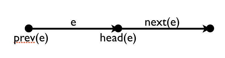
Let $x,y,z\in\mathbb{R}$ vertices and the “wrap” $g\in\mathrm{G}$ an edge. Then wie have the vertices head and tail and the edges prev and next.
component(e)

mark(e);

e' := e;

while(e'≠ e) do

e' := next(e');

if (e' == e) return true;

mark(e');

endwhile

e':=e;

while (e' ≠ NULL) do

e' := prev(e');

if(e'==e) return false;

mark(e');

endwhile
findcomponents()

num_circles :=0;

num_ints :=0;

unmark all edges;

for each edge e do

if (marked(e)) continue;

if (component(e))

then num_circles ++;

else num_ints++;

endif
Data Structure for surfaces
There are winged edges, half edges and quad edges. An oriented edge has the vertices head and tail and the faces left and right.
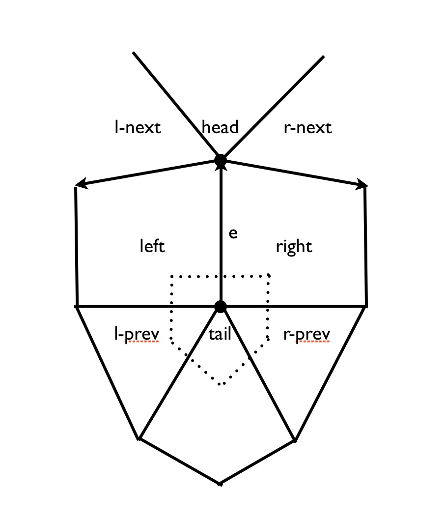
head-next(e) = – r-next(e)
head-prev(e) = – l-next(e)
tail-next(e) = – l-prev(e)
tail-prev(e) = – r-prev(e)
There is a duality: vertex $\leftrightarrow$ face, edge $\leftrightarrow$ edge ($\bot$) and face $\leftrightarrow$ vertex.
Quad edge represents both together, vertex and face are the same data structure (e.g. coordinates of vertex area of dual face). A “quad edge<2 has pointers to four vertices/faces and pointers to four other quad edges.
Store quad edge once. A reference to a quad edge is a pointer to this data structure together with two bits $±e$, $±e^+$. We need enumerators for each edge, vertex and face. and some pointers back from a vertex/face to an incident edge.
mark all edges, faces, vertices

for each edge e do

if unmarked(e)

then find_component(left(e));

end for
find_component(f)

recursively mark all neighbors (breath-first or order-first, pruning   when we see a marked face);

As we go, count faces, edges, vertices;
If we pass a marked face again with oposite direction, set a “nonorientability” flag.
Need to count components: $\chi = \mathrm{V}-\mathrm{E}+\mathrm{F}$.
With some modifications quad edges, etc. also work for multigraphs in a surface.
Similarly, for any 2-complex in $\mathbb{R}^3$ or for a 3-manifold given as a 3-complex we can use facet edge data structure.
A facet edge $f_e$ represents one edge of one face in the complex.
next_edge($f_e$), next_facet($f_e$), prev_edge($f_e$), prev_edge($f_e$)
The facet edge has four pointers to $f_e$’s, 2 pointer to vertices (head, tail) and 2 pointers to cells (above, below).
Especially when the complex forms a closed 3-manifold, we can implement duality as quad edge.
Topic: polygons, polyhedra, cell complexes and data structure for these.
$n$-manifolds looks locally like $\mathbb{E}$. Further a $n$-manifold with boundary has points with neighboorhoods like a halfspace $\{x\in \mathbb{E}^n | x_n\geq 0\}$. Compact manifolds (with boundary) are the ones that can be represented in the computer, say by a finite triangulation.
Definition: A closed $n$-manifold is a compact manifold without boundary.
Each component of a $0$-manifold is a point. The manifold is compact iff it is finite. A connected $1$-manifold is $\bigcirc\cong\mathbb{S}^1, \:\mid\:\cong [0,1],\:\updownarrow \:\cong\mathbb{R}\cong(0,1)$ or $\uparrow \:\cong\mathbb{R}_{\geq 0} \cong [0,1)$. Thus, a compact $1$-manifold has finitely many components, each is $\mathbb{S}$ or $\mathrm{I}$.
Recall: each component of a compact $2$-manifold is $\sum_{g,k}$ if orientable or $\mathrm{N}_{h,k}$ if not.
Represent a compact $1$-manifold by gluing edges together: Start with n edges and some identifications of the end points (an equivalence relation on the set of $2n$ end points). In general this gluing gives a multigraph with $n$ edges and less than $2n$ vertices. The size of each equivalence class is the degree of the resulting vertex. A finite multigraph can be realized this way iff there is no vertex of degree $0$.
Lemma: A multigraph is a $1$-manifold iff every vertex has degree $1$ or $2$.
Definition: The body is exactly the set of all vertices of degree $1$.
For $2$-dimensional manifolds (and cell complexes) we start with a finite collections of polygons and a rule for gluing edges. Equivalently, we can require that all the polygons are triangles.
Definition: An oriented $n$-gon is topologically an oriented closed disk with n marked boundary-points $a_i$ in cyclic order.
The gluing rule is an equivalence relation on the set of all oriented edges with the porperty that $e\sim f \Leftrightarrow -e \sim -f$. The equivalence classes are the oriented edges of the resulting $2$-complex.
The degree or valence of the resulting edfe is the cardinality of the equivalence class. The resulting compact space is a $2$-manifold iff all edges has valence $1$ or $2$ and edges of valence $1$ form the boundary. We get a manifold if we start with pairing of the oriented edges. The manifold is closed (no boundary) if all edges get paired.
The $2$-complex we get is always purely $2$-dimensional (no edges of valence $0$, no isolated vertices). Not every purely $2$-dimensional complex can be obtained by our construction. We’ve given a “top-down” $\:$construction of complexes. Start with to-dimensional cells gluing their face.
The other construction of cell complexes is “bottom up”.$\:$Start with a finite set of vertices. Then sew in a finite collection of edges (to head and tail vertices). Finally sew in $n$-gons by attaching boundary to a cycle of $n$ oriented edges.
With this second construction edge valence is $0$ or $2$ is necessary but not sufficient to get a manifold with boundary. We need to test that the link of each vertex is connected. Assuming the valence conditions, the link of each vertex is a $1$-manifold – we just need to check if it is $\mathrm{I}$ or $\mathbb{S}^1$.
Usually we have geometric information about how a complex is sitting in some ambient space. E.g. each vertex has coordinates. Usually edges are straight lines in the ambient space.
We may need to mark edges to say which “way around”$\:$ in the ambient space they go. If the ambient space is $\mathbb{R}^3/\:\mathrm{G}$ for some crystallographic group $\mathrm{G}$, then we often represent vertices as points $v\in\mathbb{R}^3$. An edge from $v$ to $w$ is marked with $g\in\mathrm{G}$ to show that it is the straight line $v$, $g\cdot w$ is one of the preimages.
Sometimes multiple edges are usefull even if the start in the same position.
I introduced Bezier curves and surfaces yesterday with a quick and non-technical treatment focusing on the recursive definition of the Bezier curve of order $k$ as a weighted sum of two Bezier curves of order $k-1$; the recursion is rooted in the definition that order-1 Bezier curves are line segments linearly interpolated between a pair of control points:
\[ \beta(P_0, P_1; t) := (1-t)P_1 + tP_2 \]
The definition of order-2 (quadratic) Bezier curve is then
\[\beta(P_0, P_1, P_2; t) := (1-t)\beta(P_0,P_1,t) + t\beta(P_1, P_2, t) \]
In general, one arrives at a polynomial expression in terms of the control points $P_i$ which is given for the order-n case by:
\[ \sum_{k=0}^n B_k^n(t) P_k \]
where $B_k^n(t)$ is the Bernstein polynomial defined by $B_k^n(t) := \binom{n}{k}(1-t)^kt^{n-k}$. Using this form it is not difficult to prove many attractive properties of the Bezier curves, such as: the tangent direction at $P_0$ is in the direction of $P_1$, etc.
To help you visualize the recursive definition of Bezier curves, I’ve created a demo in the SVN repository for our class. Update and run the main() method in util.BezierDemo. You’ll need to invoke the animation panel and set two key frames (by clicking on Save then Insert buttons), then hit the play button. You’ll probably want to adjust the playback speed also. Here’s a movie showing the result:

Rational Bezier curves. If one uses homogeneous coordinates for the points of space, then one can generate a wider variety of curves using the same algorithm. Remember, the final step of drawing the curve is to dehomogenize, that is, divide by the homogeneous coordinate, which in our case is the $w$-coordinate. Such a curve is then a rational rather than a polynomial curve.
Representation of circles. In particular, it is possible to parametrize arcs of circles using rational Bezier curves of degree 2. This takes advantage of the fact that the circle an be represented rationally as the homogeneous curve $(1-t^2, 2t,1+t^2)$. For $t\in [0,1]$, this parametrizes the first quadrant of the unit circle. It turns out that the Bezier curve with control points
\[ P0 := (1,0,1),~~~ P1 := \dfrac{\sqrt{2}}{2}(1,1,1), ~~~P2 := (0,1,1) \]
provides essentially the same parametrization of this circular arc.
Bezier surfaces. There are two approaches to generalizing the above approach to generate surfaces. In the first, one begins with a triangle instead of a line segment, and two parameters $u$ and $v$ instead of $t$. Then the order-1 interpolation of the triangle is defined as
\[\beta(P_0,P_1,P_2; u,v) := (1-u-v)P_0+uP_1+vP_2\]
The other approach creates surfaces as the tensor product of two curves. In this case, one requires for an order-n surface a total of $(n+1)^2$ control points. One considers these points arranged in a square array. Then to create the surface, consider each row of the array as the control points for an order-$n$ Bezier curve. Use the $u$ parameter to obtain a point on each of these curves. Then, consider these $n+1$ points as the control points of a Bezier curve, and apply the $v$ parameter to obtain a point on it. This is the value of the surface at the parameter value $(u,v)$. It’s not hard to show that one obtains the same result if one begins with the $v$ parameter and then applies the $u$.
It is well known that $\mathbb{C} \cong \mathbb{R}^2$ with
\[
z = x + y i \leftrightarrow (x,y) \leftrightarrow \begin{pmatrix}
x & – y
\\
y & x
\end{pmatrix}
=
\begin{pmatrix}
x & – y
\\
\overline{y} & \overline{x}
\end{pmatrix}
\]
Note that the multiplication rule in $\mathbb{C}$ comes from the matrix multiplication in $\mathbb{R}^{2 \times 2}$ with
\[
(x + y i)(x’ + y’ i) = (xx’ – yy’) + (xy’ + yx’)i
\]
for some $x,y,x’,y’ \in \mathbb{R}$. Of course other known operations for $x,y \in \mathbb{R}, z := x + yi$ are:
\begin{gather*}
\overline{z} = \overline{x + yi} = x – yi
\\
|z|^2 = z \overline{z} = x^2 + y^2 \in \mathbb{R}^{\ge 0}
\\
z^{-1} = \frac{\overline{z}}{|z|^2}
\\
\overline{z} = z \Leftrightarrow |z| = 1 \Leftrightarrow z \in \mathbb{S} \Leftrightarrow \begin{pmatrix}
x & – y
\\
y & x
\end{pmatrix} \in \text{SO}_2 = \{\text{special orthogonal}\}
\end{gather*}
Now consider a pair of complex numbers which will be called quaternion. Denote $\mathbb{H}$ as the set of all quaternions (named after Hamilton). Then $\mathbb{H} \cong \mathbb{C}^2 \cong \mathbb{R}^4$ with
\[
q = z + w i \leftrightarrow (z,w) \leftrightarrow
\begin{pmatrix}
z & – w
\\
\overline{w} & \overline{z}
\end{pmatrix}
\]
Accordingly we get the following rules for $z,w, z’, w’ \in \mathbb{C}, q := z + wj$:
\begin{gather*}
(z + w j)(z’ + w’ j) = (zz’ – w \overline{w’}) + (zw’ + w \overline{z’})j
\\
\overline{q} = \overline{z + wj} = \overline{z} – wj
\\
|q|^2 = q \overline{q} = |z|^2 + |w|^2 \in \mathbb{R}^{\ge 0}
\\
q^{-1} = \frac{\overline{q}}{|q|^2}
\\
\overline{q} = q \Leftrightarrow |q| = 1 \Leftrightarrow q \in \mathbb{S} \Leftrightarrow \begin{pmatrix}
z & – w
\\
\overline{w} & \overline{z}
\end{pmatrix} \in \text{SU} \cong \text{SU}_2
\end{gather*}
May think of it in a constructive way:
As a basis for $\mathbb{H}$ over $\mathbb{R}$ we can choose $\{1 , i, j, k\}$ with $k := ij$. We get
\begin{gather*}
i^2 = j^2 = k^2 = ijk = -1
\\
ij = -ji = k
\\
jk = -kj = i
\\
ki = -ik = j
\end{gather*}
The set $\{ \pm 1, \pm i, \pm j, \pm k\}$ forms a group $Q_8$, called the quaternion group of order 8.
Then we can write $q \in \mathbb{H}$ as
\[
q = t + xi + yj + zk = t + p \text{ for some } t,x,y,z \in \mathbb{R}
\]
where $p = xi + yj + zk$ is a pure (imaginary) quaternion. We denote $\text{Im}(q) := p \in \mathbb{R}^3, \text{Re}(q) := t \in \mathbb{R}$.
Identify the pure quaternions $\text{Im} \mathbb{H} := \text{span}\{ i,j,k\}$ with $\mathbb{R}$ via
\[
q \longleftrightarrow
\begin{pmatrix}
t & x & y & z
\\
-x & t & -z & y
\\
-y & z & t & -x
\\
-z & -y & x & t
\end{pmatrix}
\]
The following rules holds $t,x,y,z,t’ \in \mathbb{R},p,p’ \in \text{Im} \mathbb{H}$ with $p = xi + yj + zk$ and $q := t + p, q’ := t’ + p’$:
\begin{gather*}
\overline{q} = \overline{t + p} = t – p
\\
q \overline{q} = t^2 + x^2 + y^2 + z^2 = t^2 + |p|^2
\\
\overline{p} = -p
\\
( \overline{q} = q \Leftrightarrow t = 0 \Leftrightarrow q \in \text{Im} \mathbb{H} )
\\
q q’ = (t+p)(t’+p’) = (tt’ – p \cdot p’) + ( tp’ + t’p + p \times p’)
\end{gather*}
where $p \cdot p’$ is the common scalar product and $p \times p’$ the vector product on $\mathbb{R}^3$. In particular
\[
p p’ = – \underbrace{p \cdot p’}_{\in \mathbb{R}} + \underbrace{p \times p’}_{\in \mathbb{R}^3}, \quad – p \cdot p’ = \text{Re}(pp’), p \times p’ = \text{Im}(p p’)
\]
Any 2-dim subspace in $\mathbb{H}$ including 1 behaves like $\mathbb{C}$ (closed under the commutative multiplication). That is, given any unit pure quaternion $u \in \mathbb{S}^2 = \mathbb{R}^3 \cap \mathbb{S}^3$ the set $\{1,u\}$ spans such a 2-plane
\begin{gather*}
(x+ yu)(x’+y’u) = (xx’ – yy’) + (xy’ + yx’) u
\\
u^2 = -1
\end{gather*}
A non-real quaternion $q$ commutes only with elements of $\text{span}\{1,u\}$. $\mathbb{R} \subset \mathbb{H}$ is called the center of $\mathbb{H}$ (because the reals commute with everything). Analog to the complex setting we have $e^{\theta i} = \cos \theta + \sin \theta i$ and define
\[
e^{\theta u} := \cos \theta + \sin \theta u \quad \forall u \in \mathbb{S}^2, \theta \in \mathbb{R}
\]
For $q = t + p = t + \theta u$ we get
\[
e^q = e^t(e^{\theta u}) = e^t \cos \theta + (e^t \sin \theta)u
\]
and $e^{\theta u} \in \mathbb{S}^3$ (unit quaternions).
Claim: Any unit quaternion can be written as $e^{\theta u}$ for some $\theta \in [0, \pi], u \in \mathbb{S}^2$ (unit pure).
Indeed $\cos \theta = \text{Re}(q) \in [-1,1]$ determines $\theta \in [0,\pi]$ uniquely. Then $u = \frac{\text{Im}(q)}{|\text{Im}(q)|} = \frac{\text{Im}(q)}{\sin \theta}$ determines $u$. (Except for $\theta \in \{0,\pi\}$ since $1 = e^{0u}, -1 = e^{\pi u} \forall u \in \mathbb{S}^2$.)
These notes cover the lectures from the week of November 12 – November 15, 2012. vis_lectures_12th_15th
The euclidean plane isometry consists of 5 motions:
Suppose $G<E_2$ is a discrete group. First consider the translation subgroup of $G$. It holds $G\cap \mathbb{R}^2 < E_2$. We have
The discrete translation group forms a lattice of dimension $k= 0,1,2$.
$k=1:$ There are no translations in $G$. This implies that $G$ has a fixed point ($G$ has no glides). Thus $G<O_2$ is a finite subgroup $G=C_n$ or $D_n$ for some $n=1,2,3$. As groups of symmetries in $\mathbb{E}^2$ these are called the rosette groups or point groups since they leave at least one point fixed.
$G=C_n$ are called the cyclic group. 
The cup (first object) is $C_2$ since it has a $180^°$ symmetry. The recycling logo (2nd object) is $C_3$ and the star (3rd object) $C_5$ since the they are $120^°$ and $72^°$ symmetric. The group $C_1$ has no symmetry and can be represented by an L or an R.
$G=D_n$ are called the dihedral group.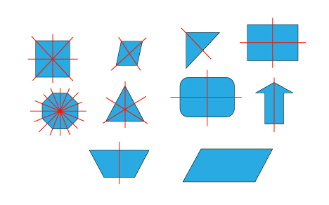
Starting with the upper left the square is $D_4$, the rhombus is $D_2$ the triangle $D_1$. The dihedral group is the group of regular polygons, so an n-gon is $D_n$.
$k=1:$ These groups are called the frieze groups. They have the following definition:
$G\cap \mathbb{R}^2 = \{ \tau_{nv} : v\neq 0 \in \mathbb{R}^2, n\in\mathbb{Z} \} = \langle \tau_v\rangle\cong \mathbb{Z}$.
$k=2:$ These groups are called the wallpaper groups. They have the following definition:
$G\cap \mathbb{R}^2 = \langle \tau_v, \tau_w\rangle \{ \tau_{nv+mw} : v,w\neq 0 \in \mathbb{R}^2, n,m\in\mathbb{Z} \} \cong \mathbb{Z}^2$.
There are seven distinct subgroups (up to scaling and shifting of patterns) in the discrete frieze group generated by a translation, reflection (along the same axis) and a 180° rotation. An overview gives the following picture 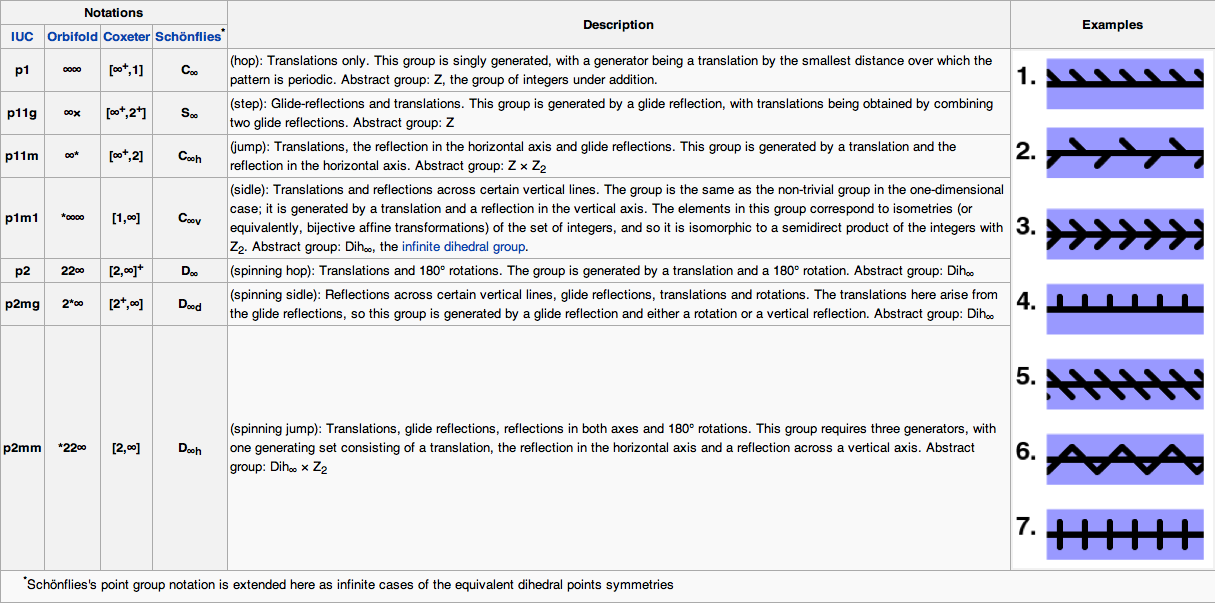
The Orbifold notation was the name we used in the lecture.
Take a width-$n$ strip $[0,n]\times\mathbb{R}\subset\mathbb{R}$ and glue its edges to give a cylinder. Any of our seven groups will give a group symmetry of the cylinder with exactly $n$-fold rotation around vertical axis. This gives $7$ families of symmetry groups, indexed by $n$. These are finite subgroups of $O_3$. They are exactly the ones that preserve the equator (or equivalent preserve the poles). These are called the axial groups:
Special cases for $n=2$:
Note that the abstract groups sometimes look different as, e.g., for the group $222$, which should have $D_2$ as its abstract group instead of $\mathbb{Z}_2$. These are equivalent because
$D_{2} \cong D_1 \times \mathbb{Z}_2 \cong \mathbb{Z}_2$.
In general, for odd $m \in \mathbb{N}$, it holds
$D_{2m} \cong D_{m} \times \mathbb{Z}_2$, and $\mathbb{Z}_{2m} \cong \mathbb{Z}_m \times \mathbb{Z}_2$.
For $n=1$, only three different groups remain:
Of course, there are more discrete subgroups of $O_3$. Most of them correspond to the symmetry groups of the platonic solids. First, we give the theorem:
Theorem: The finite subgroups of $O_3$ are the 7 families of axial groups and the 7 platonic symmetry groups $*235$, $235$ (symmetries of icosahedron and its dual, the dodecahedron), $*234$, $234$ (symmetries of the cube and the dodecahedron), $*233$, $233$ (tetrahedron), and $3*2$ (the so-called pyritohedral symmetry).
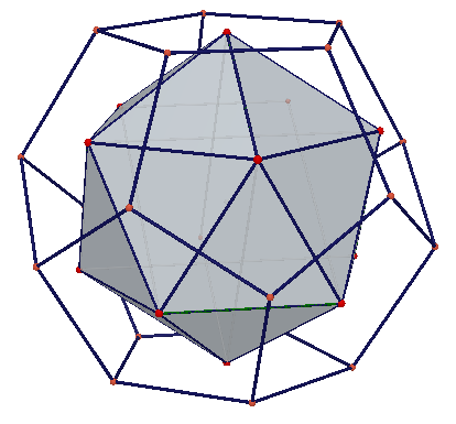
The figure on the left shows the icosahedron inside of a dodecahedron. Recall that the dual or reciprocal of a solid evolves from faces becoming vertices, roughly speaking. A symmetry of one solid is also a symmetry of its dual.
The symmetry group is $*235$, which has the rotation part $235$ as subgroup. (http://apollonius.math.nthu.edu.tw/d1/dg-07-exe/943251/dynamic/duality.htm)
 The tetrahedron has the symmetry group $*233$, with rotation subgroup $233$.
You can easily make a tetrahedron yourself by using the figure to the right, and search for the symmetry groups yourself.
Note that the tetrahedron is dual to itself.
The cube and its dual counterpart, the octahedron, have the symmetry group $*234$, and $234$. The last symmetry group, the pyritohedral symmetry group, comes as the intersection of the octahedral and the dodecahedral symmetry groups,
$3*2 = *235 \cap *234$.
In the figure below, you see a pyritohedron, which is not platonic (note that the faces are irregular pentagons).

Wallpaper groups
Back to $E_2$ (the euclidean motions in the plane), the discrete subgroups which have a translational part of dimension 2 are called wallpaper groups. In the figure below, you find an exhaustive list of the 17 wallpaper groups, each with its fundamental domain, and generating symmetries.

The 17 wallpaper groups
here you get the notes: mvsw12_lecture_2012-10-30
If there are any mistakes or ideas for improvement, post it in a comment and I gonna try to fix it.
David