Lecture 23

Proposition
We can identify the Poincaré and the Klein model by the following construction:
Consider the Klein and Poincaré disc and embed it in $\R^3$ at $x_3=0$ inside the unit sphere (cf. second picture).

Lecture23_Fig1

To obtain a point in the Poincaré model from a point in the Klein model, we do the following:

  1. Project vertically, along $e_3$, onto the upper hemisphere.
  2. Use the stereographic projection from $-e_3$ (south pole) to project the upper

hemisphere back onto the disc.

Corollary
The geodesics in the Poincaré model are circular arcs (or line segments through the origin) that intersect the unit sphere/circle orthogonally.

Lecture23_Fig2

Proof.
In the Klein model geodesics are secants. They are mapped to semicircles that intersect the boundary (the equator) orthogonally in the hemisphere.
Since the steographic projection is conformal and maps circles (or lines) to circles (or lines) the geodesics in the Poincaré disc are circular arcs that intersect the unit circle orthogonally.

Example.
For two lines construct the unique perpendicular.

Lecture23_Fig3

Remark.
On the way we constructed another conformal model of the hyperbolic space on the hemisphere.

The Poincaré half-space(/-plane) model

Consider the following map:

Lecture23_Fig4

\[\sigma\colon x\mapsto\sigma(x)=2e_2+\frac4{(x-2e_2,x-2e_2)}(x-2e_2)\,.\]
We have $\sigma(S^1+e_2)=(\R\times\{0\})\cup\infty$.
Further, $\sigma(D+e_2)=H_-^2$, where $H_-^2:=\{(x,y)^{\mathrm T}\in\R^2:y<0\}$.
By a similar calculation as the one in the proof of conformality of the Poincaré model we can show the following:

Lecture23_Fig5

\[(A,B)=\frac{16}{(p-e,p-e)^2)}(a,b)\]
by considering the map
\[\tilde\sigma\colon D\to H_1^2\,,\ p\mapsto2e_2+\frac4{(p-e_2,p-e_2)}(p-e_2)=\sigma(p+e_2)\,.\]
For the hyperbolic metric on the Poincaré model we had
\[g_p(a,b)=\frac4{(1-(p,p))^2}(a,b)=\frac{4(p-e_2,p-e_2)^2}{16(1-(p,p))^2}(A,B)=\frac1{q_2^2}(A,B)\,,\]
where $q=\tilde\sigma(p)$.

Definition
The upper half space $H_+^n:=\{x\in\R^n:x_n>0\}$ endowed with the Riemannian metric
\[g_q(A,B)=\frac1{q_n^2}(A,B)\]
where $q\in H_+^n$ and $A,B$ are tangent vectors to $H_+^n$ at $q$ is the \emph{Poincaré half-space model} of the hyperbolic space.

Properties:
This model is conformal, i.e. the angles between curves correspond to the Euclidean angles.
The geodesics are semi-circles or lines that intersect the boundary orthogonally.

Lecture23_Fig6

Lecture 22

Poincaré disc/ball model

Lecture22_Fig1

Consider the central projection with center $s$ of $H^n$ onto the plane $x_{n+1}=0$.
This map can be described by
\begin{align*}\sigma\colon H^n
&\to D=\{u\in\R^n:(u,u)<1\}\\
x&\mapsto\frac1{x_{n+1}+1}\begin{pmatrix} x_1\\\vdots\\x_n\end{pmatrix}\,.
\end{align*}
The inverse is given by
\[\sigma^{-1}(u)=\frac1{1-(u,u)}\begin{pmatrix} 2u\\1+(u,u)\end{pmatrix}\,.\]
For $s+t\left(\begin{pmatrix}u\\ 0\end{pmatrix}-s\right)=\begin{pmatrix}tu\\-1+t\end{pmatrix}$ is a point on $\vec{su}$ and
\[-1=\left\langle \begin{pmatrix}tu\\-1+t\end{pmatrix},\begin{pmatrix}tu\\-1+t\end{pmatrix}\right\rangle_{n,1}=t^2(u,u)-(t-1)^2=t^2(u,u)-t^2+2t-1\]
yields $t=0$ or $t(u,u)+2-t=0$ which is equivalent to $t=\frac2{1-(u,u)}$.
This implies $X=\begin{pmatrix}\frac2{1-(u,u)}u\\-1+\frac2{1-(u,u)}\end{pmatrix}=\frac1{1-(u,u)}\begin{pmatrix} 2u\\1+(u,u)\end{pmatrix}$.

The map $\sigma$ is the restriction of the following map to $H^n$:
\[x\mapsto s-\frac2{\langle x-s,x-s\rangle_{n,1}}(x-s)\,,\quad\text{for}\ \langle x-s,x-s\rangle_{n,1}\neq0\,.\]

Lecture22_Fig2

A point $x$ with $\langle x-s,x-s\rangle<0$ is mapped to a point on the ray $\vec{sx}$.

The plane $x_{n+1}=0$ is the orthogonal complement of $s$:
\begin{align*}\left\langle s-\frac2{\langle x-s,x-s\rangle}(x-s),s\right\rangle&=\langle s,s\rangle-\frac{2\langle x-s,s\rangle}{\langle x-s,x-s\rangle}=-1-\frac{2(\langle x,s\rangle-\langle s,s\rangle)}{\langle x,x\rangle-2\langle x,s\rangle+\langle s,s\rangle}\\&=-1-\frac{2(\langle x,s\rangle+1)}{-2-2\langle x,s\rangle}=0\,.\end{align*}
This map is an involution on the set $\{x\in\R^{n,1}:\langle x-s,x-s\rangle-1\}$ with $\sigma(H^n)=D$ and $\sigma(D)=H^n$, where $D\cong D\times\{0\}$.

Lecture22_Fig3

Theorem.
Consider two curves $\gamma_1,\gamma_2\subseteq D$ with $\gamma_1(0)=\gamma_2(0)=p\in D$ and $a:=\gamma_1′(0)$, $b:=\gamma_2′(0)$.
Let $\hat\gamma_1:=\sigma\circ\gamma_1$ and $\hat\gamma_2:=\sigma\circ\gamma_2$ be the corresponding curves in $H^n$ with $\hat\gamma_1(0)=\hat\gamma_2(0)=P=\sigma(p)$ and $A:=\hat\gamma_1′(0)$, $B:=\hat\gamma_2′(0)$.
Then:
\[\langle A,B\rangle_{n,1}=\frac4{(1-(p,p))^2}(a,b)\,.\]
This implies
\[\cosh\alpha=\frac{\langle A,B\rangle}{\sqrt{\langle A,A\rangle\langle B,B\rangle}}=\frac{(a,b)}{\sqrt{(a,a)(b,b)}}\,,\]
where $\alpha$ is the angle of intersection of $\hat\gamma_1$ and $\hat\gamma_2$.

Proof.
Calculate derivatives:
\[A=\hat\gamma_1′(0)=\frac{\mathrm d}{\mathrm dt}\left.\left(s-\frac2{\langle \gamma_1(t)-s,\gamma_1(t)\rangle}(\gamma_1(0)-s)\right)\right\vert{t=0}=-2\frac a{\langle p-s,p-s\rangle}+2\frac{2\langle p-s,a\rangle}{\langle p-s,p-s\rangle^2}(p-s)\,.\]
Similarly,
\[B=-2\frac b{\langle p-s,p-s\rangle}+2\frac{2\langle p-s,b\rangle}{\langle p-s,p-s\rangle^2}(p-s)\,.\]
Now,
\begin{align*}\langle A,B\rangle
&=\frac{4\langle a,b\rangle}{\langle p-s,p-s\rangle^2}-{2\cdot8\frac{\langle p-s,a\rangle\langle p-s,b\rangle}{\langle p-s,p-s\rangle^3}}+{16\frac{\langle p-s,a\rangle\langle p-s,b\rangle\langle p-s,p-s\rangle}{\langle p-s,p-s\rangle^4}}\\&=\frac4{(\langle p,p\rangle-2\langle p,s\rangle+\langle s,s\rangle)^2}(a,b)=\frac4{((p,p)-1)^2}(a,b)\,.\end{align*}

Definition
The open unit ball $D=\{u\in\R^n:(u,u)<1\}$ endowed with the \emph{Riemannian metric}
\[g_u(a,b)=\frac4{(1-(u,u))^2}(a,b)\,,\]
where $a$, $b$ are tangent vectors to $D$ at $u$, is the \emph{Poincaré ball model} of the hyperbolic space.
It is \emph{conformal}, i.e. the hyperbolic angles equal the Euclidean angles.

The \emph{length of a curve $\gamma\colon[0,1]\to D$} is given by
\[\operatorname{length}(\gamma)=\int_0^1\sqrt{g_{\gamma(t)}(\gamma'(t),\gamma'(t))}\mathrm dt\,.\]

Relation between Klein and Poincaré model

Lecture22_Fig4

Claim: $A$ is the vertical projection along $e_{n+1}$ of $c(x)$ onto the hemisphere:
\[A_i=c(x)_i\quad\text{for all}\ i=1,\dotsc,n\,.\]
For this, observe that $A=s+t(x-s)$ for some $t$ and $(A,A)=1$.
Thus $\left(s+t\begin{pmatrix} x_1\\\vdots\\x_{n+1}+1\end{pmatrix},s+t\begin{pmatrix} x_1\\\vdots\\x_{n+1}+1\end{pmatrix}\right)=1$ yields
\[1=1+2\left(s,t\begin{pmatrix} x_1\\\vdots\\x_{n+1}+1\end{pmatrix}\right)+t^2\left\lVert\begin{pmatrix} x_1\\\vdots\\x_{n+1}+1\end{pmatrix}\right\rVert^2\]
and hence
\[0=-2t(x_{n+1}+1)+t^2\left(\sum_{i=1}^nx_i^2+x_{n+1}^2+2x_{n+1}+1\right)\,.\]
Now by $\langle x,x\rangle=-1$ we obtain
\[t^2\sum_{i=1}^nx_i^2=t^2(x_{n+1}^2-1)\]
which gives us $t=0$ or
\[t=\frac{2(x_{n+1}+1)}{2x_{n+1}(x_{n+1}+1)}=\frac1{x_{n+1}}\,.\]
So $A=\begin{pmatrix}0\\-1\end{pmatrix}+\frac1{x_{n+1}}\begin{pmatrix} x\\x_{n+1}+1\end{pmatrix}\in\R^{n,1}$.
Thus
\[(A)_{i=1,\dotsc,n}=\frac1{x_{n+1}}x\,.\]
The coordinates of $c(x)$ are given by
\[c(x)=\begin{pmatrix}\frac1{x_{n+1}}x\\1\end{pmatrix}\,.\]
This proves the claim.

Lecture 21

Stereographic projection

Definition. Denote the unit sphere in $\mathbb{R}^{n+1}$ by $\mathbb{S}^{n}=\left\{{x \in \mathbb{R}^{n+1}|(x,x)=1}\right\}$ and its north pole by $\mathbf{N}=e_{n+1}$.
The stereographic projection is a map $\sigma\colon \mathbb{S}^{n}\to\mathbb{R}^{n} \cup \left\{{\infty}\right\}$ from $\mathbf{N}$ to the plane
$E=\left\{{x \in \mathbb{R}^{n+1}|x_{n+1}=0}\right\} \cong \mathbb{R}^{n}$ through the equator:
\[
\sigma(X)=
\left\{
\begin{array}{ll}
\infty & \textrm{, } X = \mathbf{N}\\
l_{NX}\cap E & \textrm{, } X \neq \mathbf{N}\\
\end{array}
\right.
\]
Analytically $\sigma$ is given by
\[
\sigma(X)= \sigma\ \left(\begin{pmatrix}
x_1\\\vdots\\x_{n+1}
\end{pmatrix} \right)
= \frac{1}{1-x_{n+1}}\begin{pmatrix}
x_1\\\vdots\\x_{n+1}
\end{pmatrix}
\]
since
\[N+\lambda(X-N)=e_{n+1}+\lambda \begin{pmatrix}
x_1\\\vdots\\x_{n+1}
\end{pmatrix}
= \begin{pmatrix}
y_1\\\vdots\\y_{n}\\0
\end{pmatrix}
\Rightarrow \lambda=-\frac{1}{x_{n+1}-1}=\frac{1}{1-x_{n+1}}, X\neq N.
\]

Lecture21_Fig1_1

Sphere inversion
Definition. The sphere inversion $i_{M,r}\colon \mathbb{R}^{n} \cup \left\{{\infty}\right\} \to \mathbb{R}^{n} \cup \left\{{\infty}\right\}$ in the sphere
$\mathbf{S}_{M,r}=\left\{{x \in \mathbb{R}^{n}|\left\|x-M\right\|=r}\right\}$ is given by the following conditions:

  • $X’$ lies on the ray $\overrightarrow{MX}$,
  • $\left\|M-X\right\|\left\|M-X’\right\|=r^2$,
  • $M\longleftrightarrow\infty$.

Lecture21_Fig2_1

Properties of sphere inversions

  1. $i_{M,r}$ is an involution,
  2. $\mathbf{S}_{M,r}$ is fixed,
  3. affine subspaces containing M are mapped onto themselves.


Lemma.

Lecture21_Fig3_1

Proof.
Since
\[
\left\|M-A\right\|\left\|M-A’\right\|=r^2 = \left\|M-B\right\|\left\|M-B’\right\| \iff
\frac{\left\|M-A\right\|}{\left\|M-B\right\|}=\frac{\left\|M-B’\right\|}{\left\|M-A’\right\|}
\]
we get that $\Delta AMB$ and $\Delta B’MA’$ are similar. In particular:
\[
\measuredangle MA’B’=\measuredangle ABM.
\measuredangle MAB=\measuredangle A’B’M.
\]

$\Box$

Corollary. Circles through M are mapped to lines. In particular, the line is parallel to the tangent to the circle at M.

Lecture21_Fig4_1

Remark. All lines are thought to contain the point $\infty$ and are considered as circles of infinte radius.

Corollary. The stereographic projection is the restriction of the sphere inversion $i_{M,r}$ with $M=e_{n+1}$ and $r=\sqrt{2}$.

Lecture21_Fig5_1

Proof.

  1. The equator of $\mathbb{S}^{n}$ is fixed.
  2. $\mathbb{S}^{n}$ is mapped to a plane (Corollary) through the equator (1).
  3. Both inversion and stereographic projection preserve the rays.
  4. The intersection points of a ray with $\mathbb{S}^{n}$ and $\mathbb{R}^{n}$ are unique, hence $i_{M,r}\Big|_{\mathbb{S}^{n}}=\sigma$.
  5. $N=M\longrightarrow\infty$ by $i_{M,r}$.

$\Box$

Theorem. An inversion in a sphere:

  1. maps spheres/hyperplanes to spheres/hyperplanes,
  2. is a conformal map, i.e. it preserves angles.


Lecture21_Fig6_1

Proof.
(i) Consider the following sketch:

Lecture21_Fig7_1

Hence the angles $\alpha$ and $\beta$ satisfy
\[
(\pi-\alpha)+\beta+\frac{\pi}{2}=\pi \Rightarrow \alpha-\beta=\frac{\pi}{2}.
\]
(ii) Conformality follows from the following picture

Lecture21_Fig8_1

$\Box$

Remark. In general, the center of a sphere is not mapped to the center of its image by an inversion.

Corollary.

  1. The stereographic projection maps spheres through the north pole to hyperplanes and spheres not through the north pole to spheres.
  2. All spheres/hyperplanes are images of spheres on $\mathbb{S}^{n}$ under $\sigma$ (because $i_{0,1}$ is an involution).
  3. $\sigma$ is conformal.


Formula for the sphere inversion.
Consider the second figure showing the general idea of a sphere inversion. Since $X’$ lies on the ray $XM$ we have $X’=M+\lambda(X-M), \lambda > 0$ and from the second requirement for the sphere inversion we obtain

\begin{align*}
&&\underbrace{\left\|X’-M\right\|}_{X’-M=\lambda(X-M)} \left\|X-M\right\|&=r^2\\
\Rightarrow&& \lambda \left\|X-M\right\| \left\|X-M\right\|&=r^2\\
\Rightarrow&& \lambda = \frac{r^2}{\left\|X-M\right\|^2}.
\end{align*}
Hence the sphere inversion is given by

\[
i_{M,r}=M+\frac{r^2}{\left\|X-M\right\|^2}(X-M).
\]

Lecture 20

Definition.
Let $\ell_1$, $\ell_2$ be two intersecting lines defined by unit normals $n_1$, $n_2$.
The exterior angle $\hat\alpha$ of these two lines is given by
\[\cos\hat\alpha=\langle n_1,n_2\rangle\,.\]
The interior angle $\alpha=\pi-\hat\alpha$ is given by
\[\cos\alpha=-\langle n_1,n_2\rangle\,.\]

Lecture20_Fig1

In particular, two lines are perpendicular, if $\langle n_1,n_2\rangle=0$.

Remark.
The Euclidean angle of intersection differs from the hyperbolic angle defined above.

Example
I don’t remember the example 🙁

Proposition

  1. Given $x\in H^2$ and a line $\ell\subset H^2$, there exists a unique line through $x$ perpendicular to $\ell$.
  2. If $\ell_1,\ell_2\in H^2$ are two non-intersecting lines ($\lvert \langle n_1,n_2\rangle\rvert >1$), then there exists a unique line perpendicular to $\ell_1$ and $\ell_2$.

Lecture20_Fig2

Proof. Homework.

Let $\ell_1,\ell_2\in H^2$ be two hyperbolic lines with unit normal vectors $n_1$, $n_2$:
Lecture20_Fig3

If $\lvert \langle n_1,n_2\rangle\rvert < 1$, then $\ell_1$ and $\ell_2$ intersect.

Lecture20_Fig4

If $\lvert \langle n_1,n_2\rangle\rvert = 1$, we call $\ell_1$ and $\ell_2$ parallel.

Lecture20_Fig5

If $\lvert \langle n_1,n_2\rangle\rvert >1$, we call $\ell_1$ and $\ell_2$ (ultra-)parallel.

Distances in the hyperbolic plane

Proposition
The point on a line $\ell\subset H^2$ closest to a point $x\in H^2$ is the intersection point of $\ell$ with its unique perpendicular line through $x$.

Proof.

Lecture20_Fig6

W.l.o.g. assume $x\notin\ell$.
We have
\begin{align*}
\langle n_p,x\rangle&=\langle n_p,x_p\rangle=0&
\langle n,x_p\rangle&=0&
\langle n_p,n\rangle&=0\,.
\end{align*}
We normalize $n_p$ and $x_p$ such that $\langle n_p,n_p\rangle=1$ and $\langle x_p,x_p\rangle=-1$.
Now $\gamma(s)=\cosh(s)x_p+\sinh(s)n_p$ is an arclength parametrization of $\ell$.
The distance from $x$ to $\gamma(s)$ is
\[\cosh d(x,\gamma(s))=-\langle x,\gamma(s)\rangle=-\langle x,\cosh(s)x_p\rangle-\langle x,\sinh(s)n_p\rangle=-\cosh(s)\langle x,x_p\rangle\,.\]
This is minimal for $s=0$, $\gamma(0)=x_p$.
Thus the closest point is $x_p$.

Proposition

  1. For the distance of a point $x\in H^2$ to a line $\ell\subset H^2$ defined by a unit normal $n$, we have
    \[\sinh d(x,\ell)=\lvert \langle x,n\rangle\rvert \,,\]
    where $d(x,\ell)=d(x,x_p)$ and $x_p$ is closest to $x$ on $\ell$.
  2. The distance between two non-intersecting lines $\ell_1,\ell_2\subset H^2$ with unit normals $n_1$, $n_2$ is
    \[\cosh d(\ell_1,\ell_2)=\lvert \langle n_1,n_2\rangle\rvert\,,\]
    where $d(\ell_1,\ell_2)$ is the minimal distance of two points on $\ell_1$, $\ell_2$, resp., or $d(\ell_1,\ell_2)=d(x_1,x_2)$, where $x_i=\ell_i\cap\ell_p$ and $\ell_p\perp\ell_1,\ell_2$.

Proof.
(i). Consider the arclength parametrization
\[\gamma_p(s)=\cosh(s)x_p+\sinh(s)n\]
of $\ell_p$.

Lecture20_Fig7

Now
\[x=\gamma_p(s_0)\quad\text{with}\quad s_0=\pm d(x,x_p)\,.\]
Thus
\[\lvert \langle n,x\rangle\rvert =\lvert \langle n,\cosh(s_0)x_p+\sinh(s_0)n\rangle\rvert =\lvert \sinh(s_0)\rvert \,,\]
as $n$ is normalized to $\langle n,n\rangle=1$.
This yields
\[\sinh d(x,\ell)=\sinh d(x,x_p)=\lvert \langle n,x\rangle\rvert \,.\]

(ii). Parametrize $\ell_1$ as follows:
\[\gamma_1(s)=\cosh(s)x_1+\sinh(s)n_p\,.\]
The distance of $\gamma_1(s)$ to $\ell_2$ is
\[\sinh d(\gamma(s),\ell_2)=\lvert \langle \gamma_1(s),n_2\rangle\rvert =\cosh(s)\lvert \langle x_1,n_2\rangle\rvert \]
since $\langle n_2,n_p\rangle=0$.
This is minimal for $s=0$, i.e. $x_1$ is closest to $\ell_2$ on $\ell_1$
Similarly, $x_2$ is the point closest to $\ell_1$ on $\ell_2$.
Now parametrize $\ell_p$.
\begin{align*}
x_1&=\cosh(s_0)x_2+\sinh(s_0)n_2&
x_2&=\cosh(\tilde s_0)x_1+\sinh(\tilde s_0)n_1\,.
\end{align*}
Here, $s_0=\pm d(x_1,x_2)=\pm\tilde s_0$.
Thus with $\langle n_1,n_1\rangle=1$
\begin{align*}0
&=\langle n,x_1\rangle=\cosh(s_0)\langle n_1,x_2\rangle+\sinh(s_0)\langle n_1,n_2\rangle=\cosh(s_0)\sinh(\tilde s_0)+\sinh(s_0)\langle n_1,n_2\rangle\\
&=\sinh(s_0)(\cosh(s_0)\pm\langle n_1,n_2\rangle)
\end{align*}
and hence $\cosh d(\ell_1,\ell_2)=\lvert \langle n_1,n_2\rangle\rvert $.

Intersections of $H^2$ with planes

Definition.
An affine plane is determined by one equation
\[\langle n,x\rangle_{2,1}=b\]
where $n\in\R^{2,1}$, $n\neq0$, and $b\in\R$.

Let $n$ be time-like, $\langle n,n\rangle < 0$.
If $\langle n,n\rangle=-1$, then $n\in H^2$ and $-\langle n,x\rangle=\cosh d(x,n)$ shall be equivalent to $\langle n,x\rangle=b$, i.e. the intersection of the plane given by $\langle n,x\rangle=b$ is a hyperbolic circle around $n$ with radius $r$ such that $\cosh r=-b$ ($b<0$).

Lecture20_Fig8

What are the sets defined by space-like and isotropic normal vectors?


Lecture 19

Theorem. For two points $A,B\in H_{\mathrm{pr}}^n$ let $X$, $Y$ be the points of intersection of the line $AB$ with the quadric $Q=\{[x]:\langle x,x\rangle_{n,1}=0\}$, such that $\{A,Y\}$ and $\{B,X\}$ separate each other.
Then
\[d_{\mathrm{pr}}(A,B)=\frac12\log\cr(B,X,A,Y)\,.\]

       Lecture19_Fig1

Proof.
Remember that $\cr(q,1,0,\infty)=q$.
If we choose an affine coordinate such that $X=0$, $A=1$ and $Y=\infty$, then we see that $\cr(B,X,A,Y)>1$, i.e. $\log\cr(B,X,A,Y)>0$.

Lecture19_Fig2

Parametrize $AB$ by $[a+tb]$ where $A=[a]$ and $B=[b]$.
Solving
\begin{equation}\langle a+tb,a+tb\rangle_{n,1}=0\label{ZeroesForXY}\end{equation}
yields the two solutions $t_1$, $t_2$ such that $X=[a+t_1b]$ and $Y=[a+t_2b]$.

Lecture19_Fig3

We have $t_1t_2>0$ and: If $t_1,t_2>0$ then $t_2>t_1$, i.e. $\frac{t_2}{t_1}>1$ — if $t_1,t_2<0$ then $t_1>t_2$ and thus again $\frac{t_2}{t_1}>1$.
Looking back at the equation above gives us
\[0=\langle a+tb,a+tb\rangle=\langle b,b\rangle t^2+2t\langle a,b\rangle+\langle a,a\rangle=\langle b,b\rangle(t-t_1)(t-t_2)\,.\]
Comparing the coefficients yields
\begin{align*}
2\langle a,b\rangle&=-\langle b,b\rangle(t_1+t_2)&
\langle a,a\rangle&=\langle b,b\rangle t_1t_2\,,\quad
\text{i.e}\\
t_1+t_2&=-2\frac{\langle a,b\rangle}{\langle b,b\rangle}&
t_1t_2&=\frac{\langle a,a\rangle}{\langle b,b\rangle}\,.
\end{align*}
Thus
\[\cosh d_{\mathrm{pr}}(A,B)=\frac{\lvert\langle a,b\rangle\rvert}{\sqrt{\langle a,a\rangle\langle b,b\rangle}}=\frac{\lvert t_1+t_2\rvert}{2\sqrt{t_1+t_2}}\,.\]
The cross ratio is
\[\cr(B,X,A,Y)=\cr(\infty,t_1,0,t_2)=\frac{\infty-t_1}{t_1-0}\frac{0-t_2}{t_2-\infty}=\frac{t_2}{t_1}\,.\]
This implies
\begin{align*}\cosh\frac12\log\cr(B,X,A,Y)
&=\frac12\left(\mathrm e^{\frac12\log\frac{t_2}{t_1}}+\mathrm e^{-\frac12\log\frac{t_2}{t_1}}\right)=\frac12\left(\sqrt{\frac{t_2}{t_1}}+\sqrt{\frac{t_1}{t_2}}\right)\\
&=\frac12\frac{\lvert t_2\rvert+\lvert t_1\rvert}{\sqrt{t_1t_2}}=\frac12\frac{\lvert t_1+t_2\rvert}{\sqrt{t_1t_2}}\,,
\end{align*}
since $t_1t_2>0$.

Lines in the hyperbolic plane

Hyperbolic lines are secants of the unit ball

Lecture19_Fig4

Obviously, to a line and a point in $H^2$ there exist many lines through the point that do not intersect the line:

Lecture19_Fig5

This contradicts the Parallel Axiom.

Using polarity, we can assign unit normal vectors to hyperbolic lines in $H^2$.

Lecture19_Fig6

With $\ell=P(U)$, where $U$ is a two-dimensional subspace with signature $(+-)$ (where by the signature of a subspace $V$ we denote the signature of $\langle\cdot\,,\cdot\rangle$ restricted to $V$) we have $n\in P(U^\perp)$, where $U^\perp$ has signature $(+)$ – so we can choose $n$ with $\langle n,n\rangle=1$.
For every line there exist two unit normal vectors defined via polarity with respect to $\langle\cdot\,,\cdot\rangle_{n,1}$.
There is a bijection between half planes and vectors $n\in\R^{2,1}$ with $\langle n,n\rangle=1$.

Lecture19_Fig7

Lecture19_Fig8

Proposition
Let $\ell_1,\ell_2\in H^2$ be two distinct lines in the hyperbolic plane with unit normals $n_1$, $n_2$ (i.e. $\langle n_1,n_1\rangle=1$ and $\langle n_1,p\rangle=0$ for all $p\in\ell_1$).
Then the following are equivalent:

  1. The two lines intersect.
  2. $\operatorname{span}(n_1,n_2)$ has signature $(++)$.
  3. $\lvert\langle n_1,n_2\rangle_{2,1}\rvert<1$.

Proof
(i)$\Rightarrow$(ii): Let $\ell_1\cap\ell_2=:x$.
Then $\operatorname{span}\{x\}$ has signature $(-)$, since $\langle x,x\rangle=-1$.
Thus $\operatorname{span}\{x\}^\perp$ has signature $(++)$ and $n_1,n_2\in\operatorname{span}\{x\}^\perp$.
This implies $\operatorname{span}\{n_1,n_2\}=\operatorname{span}\{x\}^\perp$ has signature $(++)$.

(ii)$\Rightarrow$(i) can be shown similarly.

(ii)$\Leftrightarrow$(iii):
The matrix for $\langle\cdot\,,\cdot\rangle\big\vert_{\operatorname{span}\{n_1,n_2\}}$ is given by
\[A=\begin{pmatrix}\langle n_1,n_1\rangle&\langle n_1,n_2\rangle\\\langle n_1,n_2\rangle&\langle n_2,n_2\rangle\end{pmatrix}=\begin{pmatrix}1&\langle n_1,n_2\rangle\\\&1\end{pmatrix}\,.\]
$A$ is positive definite if and only if $\operatorname{span}\{n_1,n_2\}$ is $(++)$, which is (ii).
But also, positive definiteness if equivalent to $1>0$ and $1-\langle n_1,n_2\rangle^2>0$, which is (iii).

Lecture 17

Hyperbolic Geometry

Lorentz Spaces

The vector space $\mathbb{R}^{p+q}$ with the bilinear form
$$ \left<x,y\right>_{p,q} = \sum_{i=1}^{p} x_i y_i – \sum_{i=p+1}^{p+q} x_i y_i $$
is the Lorentz-space $\mathbb{R}^{p,q}$. For our purposes the space $\mathbb{R}^{n,1}$ with scalar product (non-degenerate symmetric bilinear form)
$$ \left<x,y\right>_{n,1} = \sum_{i=1}^{n} x_i y_i – x_{n+1} y_{n+1} $$
is the most important case.

Reminder The orthogonal transformations are denoted by $$ O(p,q) = \{f \in GL(p+q,\mathbb{R}) \;|\; \left<f(v),f(w)\right>_{p,q} = \left<v,w\right> \;\forall v,w \in \mathbb{R}^{p+q}\}. $$
Example $\mathbb{R}^{2,1} \leadsto \mathbb{R}^3$ with $\left<x,y\right>_{2,1} = x_1y_1 + x_2y_2 – x_3y_3$

•  $\left<x,x\right>_{2,1} = x_1^2 + x_2^2 – x_3^2 = -1$

time-like vectors $\left<x,x\right>_{2,1} < 0$

•  $\left<x,x\right>_{2,1} = 0$

light-like vectors $\left<x,x\right>_{2,1} = 0$

•  $\left<x,x\right>_{2,1} = 1$

space-like vectors $\left<x,x\right>_{2,1} > 0$

Hyperbolic Spaces

Definition The $n$-dimensional hyperbolic space is
$$ H^n = \{ x\in \mathbb{R}^{n,1} \;|\; \left<x,x\right>_{n,1} = \sum_{i=1}^{n} x_i^2 – x_{n+1}^2 = -1,\; x_{n+1} > 0 \}. $$
The length of a curve $\gamma : [a,b] \rightarrow H^n$ is defined by
$$ \mathrm{length}(\gamma) = \int_a^b \sqrt{\left<\gamma'(t),\gamma'(t)\right>_{n,1}}\:dt.$$

Why is $\left<\gamma'(t),\gamma'(t)\right>_{n,1} > 0$?

The tangent space at a point $p \in H^n$ is the orthogonal complement $p^\perp$ of $p$, $\gamma : [a,b] \rightarrow H^n$ with $\gamma(t_0) = p$.
\begin{align*}\gamma \in H^n &\Longrightarrow \left<\gamma(t),\gamma(t)\right>_{n,1} = -1 \\&\Longrightarrow 2\left<\gamma(t),\gamma'(t)\right>_{n,1} = 0.\end{align*}
The scalar product of $p$ is $\left<p,p\right>_{n,1} = -1$. Construct a basis $\{p,b_1,\ldots,b_n\}$ with $\left<p,b_i\right>_{n,1} = 0$. Then the matrix of $\left<\cdot,\cdot\right>_{n,1}$ has the form
$$\left( \begin{array}{rc} -1 & 0 \\ 0 & \left( \begin{array}{cc} & \\ & \end{array} \right) \end{array} \right) \Longrightarrow \mathrm{signature}(\left<\cdot,\cdot\right>_{n,1}|_{p^\perp})\text{ is }(n,0).$$
$\leadsto$ On the tangent spaces of the hyperbolic space embedded in $\mathbb{R}^{n,1}$ we obtain a positive-definite scalar product by restricting $\left<\cdot,\cdot\right>_{n,1}$.

$\longrightarrow$ Riemannian manifolds.

We can measure angles between curves:

$$ \cos\alpha = \frac{\left<\gamma’_1(0), \gamma’_2(0)\right>_{n,1}} {\sqrt{\left<\gamma’_1(0), \gamma’_1(0)\right>_{n,1} \left<\gamma’_2(0), \gamma’_2(0)\right>_{n,1}}} $$
for $\gamma_1,\gamma_2$ in hyperbolic space.

The Hyperbolic Line

The hyperbolic line $H^1 \subset \mathbb{R}^{1,1}$ is given by $\{x\in \mathbb{R}^{1,1} \;|\; x_1^2 – x_2^2 = -1,\; x_2>0\}$. We want to measure the length of the curve $\gamma$ in $H^1$ connecting two points $p,q$.

A parametrization of $H^1 \subset \mathbb{R}^{1,1}$ is given by $\gamma : \mathbb{R} \longrightarrow H^1,\quad t \longmapsto {\sinh t \choose \cosh t}$. Then

$$\left<\gamma(t), \gamma(t)\right>_{1,1} = \sinh^2t – \cosh^2t = -1.$$
Let $p = \gamma(s_1)$ and $q = \gamma(s_2)$ where $s_1 < s_2$. Then, since $\gamma'(t) = {\cosh t \choose \sinh t}$,
\begin{align*}
\mathrm d(p,q) &= \mathrm{length}(\gamma|_{[s_1,s_2]}) = \int_{s_1}^{s_2} \sqrt{\left<\gamma'(t),\gamma'(t)\right>_{1,1}}\:dt = \int_{s_1}^{s_2} \underbrace{\sqrt{\cosh^2t – \sinh^2t}}_{=1}\:dt \\ &= s_2 – s_1.
\end{align*}
$\leadsto$ arc-length parametrization of $H^1$.

For $p$ and $q$ we have
\begin{align*}
\left<p,q\right>_{1,1} &= \left<\gamma(s_1), \gamma(s_2)\right>_{1,1} \\
&= \sinh s_1\sinh s_2 – \cosh s_1\cosh s_2 \\
&= -\cosh(s_2 – s_1) \\ \\
\Longrightarrow \cosh(\mathrm d(p,q)) &= – \left<p,q\right>_{1,1} \\
\mathrm d(p,q) &= \mathrm{arcosh}(-\left<p,q\right>_{1,1}).
\end{align*}

Hyperbolic lines in $H^n$

Definition A hyperbolic line in $H^n$ is the non-empty intersection of $H^n$ with a 2-dim. subspace $U$ of $\mathbb{R}^{n,1}$.

Proposition The restriction of $\left<\cdot,\cdot\right>_{n,1}$ to $U$ has signature $(+-)$.

Proof Since $U \cap H^n\ne\emptyset$ there exists $u\in U$ with $\left<u,u\right> = -1$. Let $\{u,v\}$ be a basis of $U$. Define $$w = v + \left<v,u\right>u = v – \frac{\left<v,u\right>}{\left<u,u\right>}u.$$
Then
\begin{align*}
\left<u,w\right> &= \left<u,v\right> + \left<v,u\right>\underbrace{\left<u,u\right>}_{-1} = 0 \\ \\
\Longrightarrow& w\in u^\perp \\
\Longrightarrow& \left<w,w\right> > 0
\end{align*}
since the signature of $\left<\cdot,\cdot\right>|_{u^\perp}$ is $(++\ldots+)$.

$\Box$

So we can identify $H^n \cap U \subset \mathbb{R}^{n,1}$ naturally with $H^1 \subset \mathbb{R}^{1,1}$.

Lecture 16

Quadrics

Definition. Let $q$ be a quadratic form on $\mathbb{R}^n$ or $\mathbb{C}^n$. Then the corresponding quadric is $Q = \{[v] \in \RP^n \mid q(v) =0\}$

A conic is a quadric in $\RP^2$.

How many indefinite non-degenerate quadratic forms exists in $\mathbb{R}^{n+1}$ up to change a basis?

Classification by the signature: (+++..+), (+++..+ -), …, (+ – …-), (- – – ..-), should be indefinite $\Rightarrow$ n indefinite quadrtic forms (+++..+ -), … , (+ – …-).

The number of non-empty non-degenerate quadrics in $\mathbb{R}P^n$ is $\lceil \frac{n}{2} \rceil$

Example

$n=2$: In $\RP^2$ there exist only one indefinite non-degenerate quadric/conic up to projective transformations. It has signature ( + + – ) resp. ( – – +).

$n=3$: In $\RP^3$ there exist $\lceil \tfrac32 \rceil = 2$ different quadrics up to projective transformations:

  1.  (+ + + – ), ( – – – +), $Q_1 = \{[v] \in \mathbb{R}P^3 \mid v_1^2 + v_2^2 + v_3^2 – v_4^2 = 0 \}$
  2.  ( + + – – ), ( – – – +),  $Q_2 = \{[v] \in \mathbb{R}P^3 \mid v_1^2 + v_2^2  –  v_3^2  –  v_4^2 = 0 \}$

Lecture16_Fig2

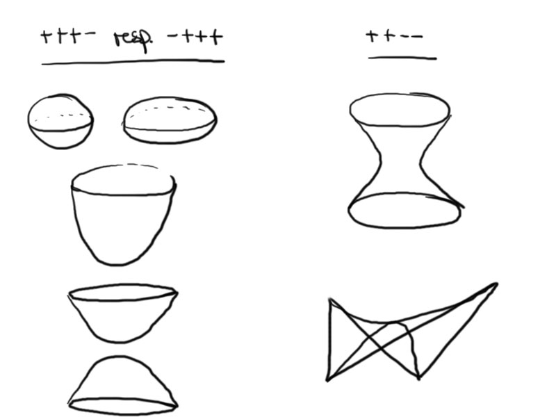
1. is a unit sphere (or ellipse, paraboloid or 2-sheeted hyperboloid) depending on the choice of affine coordinate. To obtain a sphere as affine image of the quadric we can choose the affine coordinates  $u_1 = \frac{v_1}{v_4}$, $u_2 = \frac{v_2}{v_4}$, and $u_3 = \frac{v_3}{v_4}$.

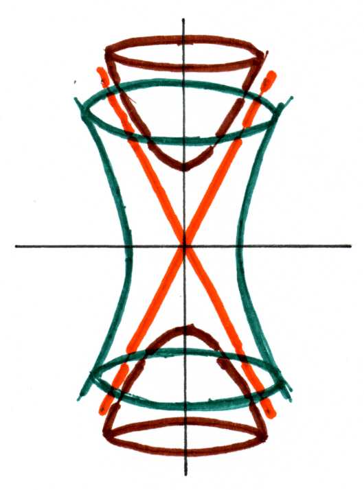
2. is one-sheeted hyperboloid or hyperbolic paraboloid.

Degenerate Quadratic forms/quadrics.

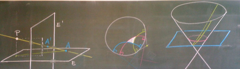
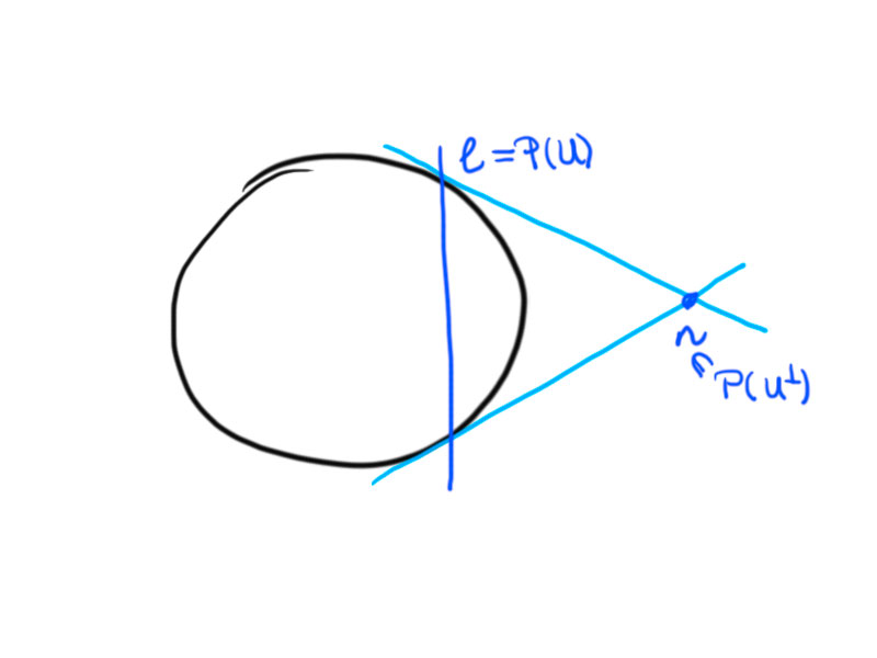
Let b be a degenerate bilinear form. Then the space $\{ u \in U \mid b(u, v) = 0 \forall v \in V \} = \ker(b) $ is a subspace of $V$. Consider a subspace $U_1 \subset V$ such that $V = \ker(b) \oplus U_1$, then $b\mid_{U_1}$ defines a non-degenerate quadric $Q_1$ in $P(U_1)$. The quadric $Q$ defined by $b$ is the union of lines through points in the non-degenerate quadric $Q_1$ defined by $b|_{U_1}$ and points in $ P(\ker(b))$ if $Q_1 \neq \emptyset$ (see Exercise 8.1).

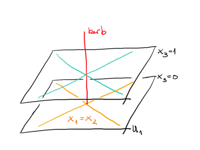
Example of degenerate conic.

Consider the following bilinear form in $\mathbb{R}P^2$:

\[
b (\begin{pmatrix} x_1\\  x_2\\x_3\end{pmatrix} , \begin{pmatrix} x_1\\ x_2\\ x_3\end{pmatrix}) = {x_1}^2 – {x_2}^2.
\]

Then $\ker (b) = span \{e_3\}$ and $\mathbb{R}^3 = \ker(b) \oplus \underbrace {span\{e_1, e_2\} }_{U_1}$.  Projectively, $P(\ker(b))$ is a point and the quadric defined by $b|_{U_1}$ in $P(U_1)$ consists of two points. So the degenerate/singular conic definined by $b$ in $\RP^2$ consists of two crossing lines.

Lecture16_Fig1

Proposition. A non-degenerate non-empty quadric $Q \subset \RP^n$ determines the corresponding bilinear form up to a non-zero scalar multiple.

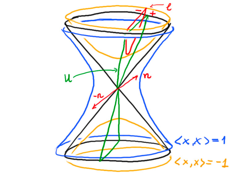
Proof. Let $b$  and $\tilde b$ be two linear forms defining $Q$. Consider an orthonormal basis w.r.t. $b$, i.e. $\{ e_1 .. e_p, f_1 .. f_q \} $, such that:

  1. $b(e_i, e_i) = 1$ for all $i = 1, \ldots, p$;
  2. $b(f_j, f_j) = -1$ for all $j = 1, \ldots, q$; and
  3. $b(e_i, e_k) = b(f_j, f_l) = b(e_i, f_j) = 0$ for all
    $i, k = 1, \ldots, p$ with $i \neq k$ and
    $j, l = 1, \ldots, q$ with $j \neq l$.

Consider the vectors $e_i \pm f_j$. Then

\begin{align*}
& b( e_i \pm f_j, e_i \pm f_j) = \underbrace{b(e_i, e_i)}_{=1} \pm \underbrace{2b(e_i, f_j)}_{=0} + \underbrace{b( f_j, f_j)}_{-1} = 0 \\
\Rightarrow& 0 = \tilde b( e_i \pm f_j, e_i \pm f_j) =  \tilde b(e_i, e_i) \pm \tilde 2b(e_i, f_j) + \tilde b ( f_j, f_j)\\
\Leftrightarrow& \pm 2 \tilde b (e_i, f_j) = – \tilde b(e_i, e_i) – \tilde b(f_j, f_j) \\
\Rightarrow& \tilde b (e_i, f_j) = 0 \\
\Rightarrow& \tilde b(e_i, e_i) = – \tilde b (f_j, f_j).
\end{align*}

So setting $\tilde b (e_1, e_1) = \lambda \neq 0$ implies that $\tilde b(e_i, e_i) = \lambda$ for all $i = 1, \ldots, p$ and $\tilde b(f_j, f_j) = – \lambda$ for all $j = 1, \ldots, q$.


Orthogonal Transformations

Definition. Let $b$ be a non-degenerate symmetric bilinear form on $\mathbb{R}^{n+1}$. Then $F: \mathbb{R}^{n+1} \rightarrow \mathbb{R}^{n+1} $ is orthogonal (wrt. $b$) if $ b(F(v), F(w)) = b(v,w) \forall v,w \in \mathbb{R}^{n+1}$.

The group of orthogonal transformations for a bilinear form of signature $(p, q)$ with $p+q = n+1$ is denoted by $ O(p,q)$. If $q=0$ we obtain the “usual” group of orthogonal transformations $O(n+1) = O(n+1, 0)$

If $Q \subset \RP^n$ is a non-degenerate quadric defined by $b$ and  $F: \mathbb{R}^{n+1} \rightarrow \mathbb{R}^{n+1} $ is an orthogonal transformation, then the map $f: \mathbb{R}P^n \rightarrow \mathbb{R}P^n$ with $[x] \mapsto f([x]) = [F(x)]$ maps the quadric onto itself: $f(Q) = Q$.

Proposition. If the signature of a non-degenerate quadric $Q$ is $(p,q)$ with $p \neq q$ and $p \neq 0 \neq q$, then any projective transformation with $ f(Q) = Q$ is induced by an orthogonal transformation $F$ w.r.t. $b$ that defines $Q$.

Proof. Let $b$ be the bilinear form defining $Q$ and $F$ the linear transformation defining the projective transformation $f$. Then $\tilde b(v,w):= b(F(v), F(w))$ is another bilinear form defining $Q$.

According to the previous proposition there exists $\lambda \neq 0$ such that

\[b=\lambda \tilde b.\]

If $\lambda > 0 $ then $\frac{1}{\sqrt \lambda} F$ is an orthogonal transformation, since $ b( \frac{1}{\sqrt \lambda} F(v), \frac{1}{\sqrt \lambda} F(w)) = \frac{1}{\lambda} b (F(v), F(w)) = \frac{1}{\lambda}\tilde b (v,w) = b(v,w)$.

So we need to show that $\lambda > 0$.

If $\{ e_1, \ldots, e_{n+1}\}$ is an orthogonal basis of $\mathbb{R}^{n+1}$ w.r.t. $b$ then $\{F(e_1), \ldots, F(e_{n+1}\}$ is also orthogonal with

  • If $b(e_i, e_i) = 1$ then $\tilde b(e_i, e_i) = \lambda$
  • $b(e_i, e_i) = -1 \Rightarrow \tilde b(e_i, e_j) = – \lambda$.

But the signature is invariant w.r.t. to change of basis (i.e. w.r.t. F). So since $ p \neq q$ we have that the $\lambda $ is positive. $\square$

If $p = q$ (neutral signature), for example $p=q=2$ for a quadric  in $\RP^3$, then there exists a projective transformation preserving the quadric not induced by an orthogonal transformation. Let $b(x,x) = {x_1}^2 + {x_2}^2 – {x_3}^2 – {x_4}^2$. Then the map:

\[
f : \RP^3 \rightarrow \RP^3 ,
\sqvector{x_1\\x_2\\x_3\\x_4}
\mapsto
\sqvector{x_3\\x_4\\x_1\\x_2}
\]

yields $b(F(v), F(w)) = – b (x,x) = {x_3}^2 + {x_4}^2 – {x_1}^2 – {x_2}^2$. So $f$ preserves the quadric but it is not induced by an orthogonal transformation $F$.


Lecture 15

Pole-Polar Relationship

  • b is non-degenerate symmetic bilinear form (e.g.scalar product on $\mathbb{R}^n$)
  • orthogonal complement of a vector subspace $U\subseteq V$
    \[U^{\perp}= \left\lbrace v\in V\mid b\left(u,v\right) = 0,\forall u\in U\right\rbrace \]
  • $dimU^{\perp} + dim U = dim V$, but $U^{\perp} \oplus U \neq V$.
  • If $P\left( U\right)$ is a projective subspace of $P\left(V\right)$,then $P\left(U^{\perp}\right)$ yields another subspace of $P\left(V\right)$.
  • in $\RP^2 = P(\mathbb{R}^3)$ we obtain:
    Point $\left[ P\right] \leftrightarrow$ line $P\left( \left\lbrace p\right\rbrace ^{\perp}\right)$
    Line $P\left( U\right)\leftrightarrow$ point $P\left(U^{\perp}\right)$

Continue reading

Lecture 14

Polarity: Pole – Polar Relationship

Let $b: V \times V \rightarrow \mathbb{F}$ be a symmetric non-degenerate bilinear form.

Definition. Let $U \leq V$ be a vector subspace. Then

\[
U^{\perp} = \{ v \in V \: | \: b(u,v) = 0, \: \forall u \in U \}.
\]

If $U = \{u_1,…,u_k\}$ then

\[
U^{\perp} = ( \text{span} \; U )^{\perp} = \{ v \in V \: | \: b(u_i,v) = 0, \: \forall i = 1,…,k \}.
\]

We call $U^{\perp}$ the orthogonal complement of $U$.

Remark. dim $U^{\perp} =$ dim $U^0 = n – k$, if dim $U = k$ and dim $V = n$.

Continue reading