
Roughly speaking, Combinatorial complexes play a similar role in the discrete world as differentiable manifolds in the smooth world. They are able to capture the “intrinsic” properties of a geometric object, i.e. those properties that are independent of any embedding into an ambient space. Combinatorial complexes come in two flavors: cell complexes and simplicial complexes. In this post we deal with the former.
A one-dimensional combinatorial cell complex is the same thing as a finite multigraph. Such a multigraph $M$ is given by
- a finite set $P$ of “points”.
- a finite set $\tilde{E}$ of “oriented edges”.
- maps $s,d: \tilde{E}\to P$ assigning to each oriented edge its “source point” $s(e)$ and its destination point $d(e)$.
- a map $\rho: \tilde{E}\to \tilde{E}$ that implements “orientation reversal”: We demand that for all $e\in\tilde{e}$ we have $\rho(e)\neq e$ and $\rho\circ \rho(e)=e$. Moreover we assume
\begin{align}s\circ \rho &= d \\ d\circ \rho &= s.\end{align}
Note that what we call “points” usually would be called “vertices”. We use “points” in order to remain consistent with Houdini terminology. A two-element subset $\hat{e}\subset\tilde{E}$ of the form $\{e,\rho(e)\}$ is called an (unoriented) edge of $M$.
A typical multigraph looks like this:
You see that there can be several edges connecting the same pair of points and there can be oriented edges whose source and destination point coincide. There also could be isolated points that do not belong to any edge.
A two-dimensional combinatorial cell complex is a one-dimensional cell complex $G$ together with a set $F$ of faces, where to each face $\varphi$ there is assigned a corresponding “edge cycle” of $G$. What is an edge cycle?
An edge loop in a one-dimensional cell complex $G$ is a finite sequence $(e_1,\ldots,e_n)$ of oriented edges in $G$ such that for $1\leq j\leq n$ we have
\[d(e_j)=s(e_{j+1})\]
and $d(s_n)=s(e_1)$. An oriented edge cycle in $G$ is an equivalence class of edge loops where two edge loops are considered equivalent if they only differ by a cyclic permutation of the edges. Similarly, we obtain an unoriented edge cycle (or briefly an edge cycle) if we also allow reversing the order of the loop.
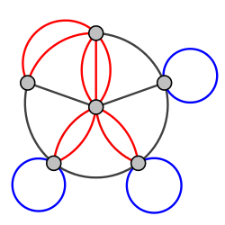
$G$ is called the 1-skeleton of the two-dimensional combinatorial cell complex $M$. Here is a visualization of a two-dimensional combinatorial cell complex with five vertices, ten edges and six faces:
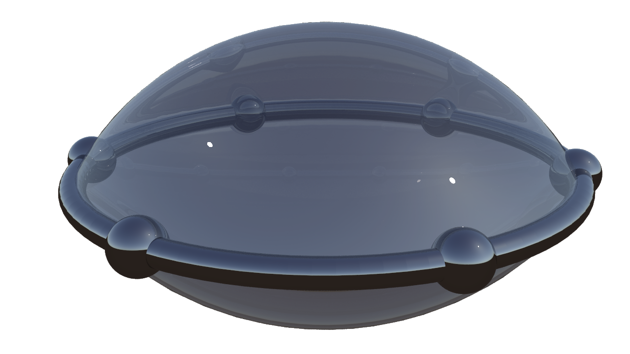
 Note that different faces can have the same edge cycle. This is for example the case for the sphere below, which is represented as a two-dimensional cell complex with six points, six edges and two faces:
A two-dimensional combinatorial cell complex $M$ can be considered as a description of a certain topological space $\hat{M}$, a so-called two-dimensional cell complex. An $n$-dimensional cell is just the unit ball $B^n\subset \mathbb{R}^n$, considered as a topological space.
- The points $p\in P$ of a two-dimensional combinatorial cell complex the represent $0$-cells. This cloud $P$ of isolated points is called the $0$-skeleton $\hat{M}_0$ of the cell complex $\hat{M}$.
- Each edge $e\in E$ corresponds to a copy of the intervall $[-1,1]$ (the unit ball in $\mathbb{R}^1$). The end points of this 1-cell are identified with the end points of $e$ prescribed by the combinatorics. The topological space that results from this gluing is called the $1$-skeleton $\hat{M}_1$ of $\hat{M}$.
- Corresponding to each face $\varphi\in F$ we have a $2$-cell $c_\varphi$, i.e. a copy of the unit disk $B^2\subset \mathbb{R}^2$. The boundary $\partial c_\varphi$ of each $1$-cell is homeomorphic to the unit circle $S^1$. Up to topological equivalence there is a unique map of $\partial c_\varphi$ to the $1$-skeleton $\hat{M}_1$ that fits the edge cycle of $\varphi$. The space obtained from gluing in this way the boundaries of all $2$-cells to the 1-skeleton $\hat{M}_1$ finally is the 2-dimensional cell complex $\hat{M}$.
See the Wikipedia articles on abstract cell complexes and CW-complexes for further information.
Two-dimensional combinatorial cell complexes are very common in Computer Graphics. In particular, what usually is called a “polygonal surface” is a two-dimensional combinatorial cell complex $M$ together with a map $P\to \mathbb{R}^3$ that gives each point a position in space.
Note however that it is not even clear how to render a face $\varphi$ of such a polygonal surface if the points on the boundary cycle of $\varphi$ are positioned on a plane. The same problem arises for numerical computations in the spirit of finite elements that need to extend quantities given on the boundary of a face to its interior. This is the reason why for many practical applications simplicial complexes are more adapted than cell complexes. We will study these in the next post.