In this tutorial we want to construct Hopf cylinders and Hopf tori. These are flat surfaces in \(\mathrm S^3\) and allow for an easy conformal parametrization when mapped to Euclidean 3-space by stereographic projection. For tori we will encounter a problem similar to the problem we saw for framed curves – there is a certain angle defect. Adjusting the immersion destroys the conformality, but we can ask for a minimal distortion.
The 3-sphere admits a fibration into circles, i.e. there is a map \(\pi\colon \mathrm S^3 \to \mathrm S^2\) such that for each point \(p\in\mathrm S^2\) there is a neighborhood \(U\subset \mathrm S^2\) such that its preimage \(\pi^{-1}(U)\) looks like the product \(U\times \mathrm S^1\):\[\pi^{-1}(U)\cong U\times \mathrm S^1.\]In particular, for each point \(p\) the fiber \(\pi^{-1}(\{p\})\) is just a circle.
Let us consider the 3-sphere \(\mathrm S^3\) to sit in \(\mathbb H\), i.e. \(\mathrm S^3 = \{\psi\in \mathbb H \mid |\psi| = 1\}\). As usual we identify \(\mathbb R^3\) with the purely imaginary quaternions. The 2-sphere is then just intersection of \(\mathrm S^3\) with \(\mathbb R^3\), \(\mathrm S^2 = \mathrm S^3\cap\mathbb R^3\), and the Hopf fibration \(\pi\colon \mathrm S^3 \to \mathrm S^2\) is given by\[\psi \mapsto \psi\,\mathbf i\,\overline{\psi}.\]In other words, it sends a quaternion to the point it rotates the vector \(\mathbf i\) to. In particular it is clear that the image is the whole 2-sphere. Similarly, the preimage of a point \(p\) consists of all rotations that rotate \(\mathbf i\) to the point \(p\). Certainly there are many such – e.g. we can precompose any rotation around \(\mathbf i\). One can check that these are in fact all: For \(\psi_o\in\pi^{-1}(\{p\})\), \[\pi^{-1}(\{p\}) = \{\psi_0e^{\mathbf i \,\alpha}\mid \alpha \in \mathbb R\} = \psi_0 \mathrm S^1,\]where \(\mathrm S^1 = \{x+\mathbf i y \in \mathbb H \mid x^2+y^2 = 1\}\). In particular the fibers are great circles in \(\mathrm S^3\).
Just to note here, \(\mathrm S^3\) forms group (multiplication is inherited from the multiplication in \(\mathbb H\)), which contains \(\mathrm S^1\) as a subgroup. The corresponding group action \[\mathrm S^3\times\mathrm S^1 \mapsto \mathrm S^3, \quad(u,\psi)\mapsto \psi u.\]maps the fibers of \(\pi\) onto itself.
Further we will need that the differential \(d\pi\) preserves the product and in particular the length of tangent vectors which are perpendicular to the fibers: Suppose that \(\psi\colon(-\varepsilon,\varepsilon)\to \mathrm S^3\) is a curve in the fiber over a point \(p\in\mathrm S^2\), i.e. \(\pi(\psi(t)) = p\) for all \(t\in(-\varepsilon,\varepsilon)\) with \(\psi(0)=\psi_0\). Then \(\psi\) is of the form\[\psi(t) = \psi_0e^{\mathbf i \alpha(t)},\] where \(\alpha\) is some real-valued function with \(\alpha(0)=0\). Taking the derivative at \(t=0\) yields\[\psi^\prime(0) =\psi_0(e^{\mathbf i \alpha})^\prime(0) = \psi_0\mathbf i \alpha^\prime(0).\]
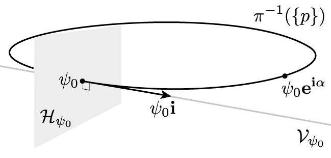
Since \(\psi\) was arbitrary, we see that the vertical space \(\mathcal V_{\psi_0}\) at a point \(\psi_o\), i.e. the tangent space of the fiber at \(\psi_0\) is given as follows\[\mathcal V_{\psi_0} = \bigl\{ X \in \mathbb H \mid X = \psi_0 \mathbf i\, x, \, x\in \mathbb R\bigr\} =\psi_0 \mathbf i \mathbb R.\]The horizontal space \(\mathcal H_{\psi_0}\) is then defined to be the orthogonal complement of \(\mathcal V_{\psi_0}\):\[\mathcal H_{\psi_0} = \bigl\{X \in \mathrm T_{\psi_0} \mathrm S^3 \mid X \perp \mathcal V_{\psi_o} \bigr\} =\bigl\{X \in \mathbb H \mid X \perp \psi_0,\psi_o\mathbf i \bigr\}.\]Note that, since we are speaking about tangent vectors to the 3-sphere at the point \(\psi_0\), \(X\) must be perpendicular to \(\psi_0\) as well.
Theorem 1. The restriction of differential \(d_{\psi_0}\pi\) to \(\mathcal H_{\psi_0}\) preserves the metric (up to a factor of \(4\)): For all \(X,Y\in \mathcal H_{\psi_0}\),\[\langle d_{\psi_0}\pi\,(X),d_{\psi_0}\pi\,(Y)\rangle = 4\langle X,Y\rangle.\]
Proof. First, we compute the differential of \(\pi\): For each tangent vector \(X\in \mathrm T_{\psi_0}\mathrm S^3\) there is a curve \(\gamma\colon (-\varepsilon , \varepsilon) \to \mathrm S^3\) such that \(\gamma(0)=\psi_0\) and \(\gamma^\prime(0) = X\). With the usual product rule we get \[d_{\psi_0}\pi\,(X)=(\pi\circ\gamma)^\prime(0) = \gamma^\prime(0)\mathbf i\, \overline{\gamma(0)} + \gamma(0)\mathbf i\, \overline{\gamma^\prime(0)} =X\mathbf i\,\overline{\psi_0} + \psi_0\mathbf i\,\overline{X}.\]Now we proceed in two steps: First we look at the differential at \(\psi_0 = \mathbf 1\). Then we have \(X\in \mathcal H_{\mathbf 1}\) if and only if \(X \in\mathrm{span}\{\mathbf j, \mathbf k\}\). In particular, such \(X\) anti-commute with \(\mathbf i\). Note also that \(\mathcal H_{\mathbf 1}\subset\mathbb R^3\). Thus we for \(X \in \mathcal H_{\mathbf 1}\) that \[d_{\mathbf 1} \pi\, (X) = X\mathbf i + \mathbf i\, \overline{X} = X\mathbf i + X\mathbf i = 2X \mathbf i.\]Now, let \(\psi_0\) be an arbitrary point on \(\mathrm S^3\) and \(X\in \mathcal H_{\psi_0}\). Then again there is a curve \(\gamma\) such that \(\gamma(0) = \psi_0\) and \(\gamma^\prime(0) = X\). Now, define \(\tilde\gamma:=\overline{\psi_0}\gamma\) or, equivalently, \(\gamma = \psi_0\tilde\gamma\). Then \(\tilde\gamma\) is a curve on \(\mathrm S^3\) through the point \(\mathbf 1\). Hence \(\tilde X :=\tilde\gamma^\prime(0)\in \mathrm{T}_{\mathbf 1}\mathrm{S}^3\). Now,\[\pi\circ\gamma = \gamma\,\mathbf i\, \overline{\gamma} = \psi_0 \,(\pi\circ\tilde\gamma)\,\overline{\psi_0}.\]Hence we obtain\[d_{\psi_0}\pi\,(X) = (\pi\circ\gamma)^\prime(0)=\psi_0 \,(\pi\circ\tilde\gamma)^\prime(0)\,\overline{\psi_0} =\psi_0 \,d_{\mathbf 1}\pi\,(\tilde X)\,\overline{\psi_0}.\]Further, we have \(\tilde X = \tilde\gamma^\prime(0) = \overline{\psi_0}\gamma^\prime(0) = \overline{\psi_0}X\). In particular \(\tilde X \in \mathcal H_{\mathbf 1}\). Thus we obtain\[d_{\psi_0}\pi\,(X) =\psi_0 \,d_{\mathbf 1}\pi\,(\tilde X)\,\overline{\psi_0} =\psi_0 2\tilde X \mathbf i\,\overline{\psi_0} =2X \mathbf i\,\overline{\psi_0}.\]But multiplication by quaternions of unit length are isometries of \(\mathbb H\): If \(\psi\in\mathrm S^3\) and \(X,Y\in\mathbb H\), then \[\langle X\psi, Y\psi\rangle =\langle X, Y\rangle =\langle \psi X, \psi Y\rangle.\]The last to statements together prove the claim.\(\square\)
Now, if \(\gamma \colon [0,L] \to \mathrm S^2\) with \(\left|\gamma^\prime\right| =1\), then the preimage \(\mathrm M\) of \(\gamma\) is a family of great circles in \(\mathrm S^3\), i.e. a cylinder. This cylinder can be parametrized as follows: Given a lift \(\psi_0\) of \(\gamma\), i.e. a curve \(\psi_0\colon [0,L]\to \mathrm S^3\) such that \(\gamma = \pi\circ \psi_0\), then a parametrization is given by\[f_0\colon [0,L] \times \mathbb R/2\pi\mathbb Z\to \mathrm S^3,\quad (t,\alpha)\mapsto \psi_0(t)e^{\mathbf i \alpha}.\]Certainly, there are many possibilities to lift \(\gamma\): It is not hard to see that any other lift \(\psi\) of \(\gamma\) is of the form \[\psi = \psi_0 g,\]where \(g\colon [0,L]\to \mathrm S^1\). This \(\psi\) then defines another parametrization, say \(f\). Our goal is to end up with an isometric immersion, i.e. we want \[\Bigl|\frac{\partial f}{\partial t}\Bigr| = 1 =\Bigl|\frac{\partial f}{\partial \alpha}\Bigr|,\quad \frac{\partial f}{\partial t} \perp\frac{\partial f}{\partial \alpha}.\]Let us compute the derivative of \(f\) with respect to \(\alpha\):\[\frac{\partial f}{\partial \alpha} = \psi_0\frac{\partial }{\partial \alpha}e^{\mathbf i \alpha}=\psi_0 e^{\mathbf i \alpha}\mathbf i.\]Thus by constrution, we always have that \(\bigl|\frac{\partial f}{\partial \alpha}\bigr|=\bigl|\psi_0\bigr|=1\). The derivative with respect to \(t\) is basically given by the derivative of the lift \(\psi\):\[\frac{\partial f}{\partial t}(t) = \psi^\prime (t)e^{\mathbf i\alpha}.\]Hence we see that \(\frac{\partial f}{\partial t} \perp\frac{\partial f}{\partial \alpha}\) if and only if \(\frac{\partial \psi}{\partial t}(t)\in \mathcal H_{\psi(t)}\). Such a lift is called a horizontal lift. Now, let \(\psi\) be a horizontal lift. Then, with the Theorem 1, we get:\[\bigl|\psi^\prime\bigr| =\tfrac{1}{2}\bigl|d_{\psi}\pi(\psi^\prime)\bigr| = \tfrac{1}{2}\bigl|(\pi\circ\psi)^\prime\bigr| = \tfrac{1}{2}\bigl|\gamma^\prime\bigr|.\]This then can be fixed by changing the parameter \(t\). We collect the facts in the following
Theorem 2. Let \(\gamma\colon [0,L/2] \to \mathrm S^2\) such that \(|\gamma^\prime| = 2\) and let \(\psi\) be a horizontal lift to the 3-sphere. Then the map\[f\colon [0,L/2]\times\mathbb R/2\pi \to \mathrm S^3, \quad (t,\alpha)\mapsto \psi(t)e^{\mathbf i\alpha}\]is an isometric parametrization of the Hopf cylinder defined by \(\gamma\).
Remark. Suppose that \(\gamma\colon \mathbb R \to \mathrm S^2\) is periodic. Then the preimage forms a torus instead of a cylinder. Assuming that \(|\gamma^\prime|=2\) the parameterization in Theorem 2 still yields an isometric immersion. But the immerison does not need to be periodic in \(t\): Let us look at the horizontal lift \(\psi\). If \(L/2\in \mathbb R\) denotes the period of \(\gamma\), we find that\[\pi(\psi(0)) = \gamma(0) = \gamma(L/2) = \pi(\psi(L/2)).\]Thus \(\psi(0)\) and \(\psi(\omega)\) both are points in the fiber over \(\gamma(0)\), thus there is \(r\in \mathrm S^1\) such that\[\psi(\omega) =\psi(0)r.\]But there is no reason why \(r\) should be equal to \(\mathbf 1\). If we want to obtain a doubly periodic immersion we must drop that \(\psi\) is horizontal. In fact one can do this similarly as for the framed curves: Let \(\omega\in (-\pi,\pi]\) such that \(r=e^{\mathbf i\omega}\) and let \(\psi\) be a horizontal lift of \(\gamma\). Then we define\[\tilde\psi(t)= \psi(t)e^{-\mathbf i\, \omega t}.\]Then \(\tilde\psi\) is a closed lift of \(\gamma\) to \(\mathrm S^3\) that will produce an immersion which not isometric but has a constant shear. Since we piked \(\omega\) between \(-\pi\) and \(\pi\) it is least shear we can choose – unless we allow for covering \(\gamma\) several times.
Now let us switch to the discrete setup. Here we start with a discrete curve \(\gamma\) on the 2-sphere and want to come up with a parametrization of the corresponding Hopf cylinder.
A discrete curve on the 2-sphere is just a finite sequence of points on \(\mathrm S^2\). In \(\mathbb R^3\) one imagines that these points are connected by straight lines. Though Houdini will visualize these curves also using straight edge segments in \(\mathbb R^3\) it seems natural to imagine that the points of a spherical curve are actually connected by great circles arcs – the shortest paths on the sphere. Unless the edge doesn’t connect antipodal points this will cause no trouble.
The horizontal lift played an important role in the smooth theory. So we should come up with a discrete analogue. One should notice that the horizontal lift along a curve can actually be regarded as a transport from fiber over the start point to the fiber over the end point of the curve: Given a curve \(\gamma\colon [0,1]\to \mathrm S^2\) and a point \(\psi_0\) in the fiber over \(\gamma(0)\), then there is a unique horizontal lift \(\psi\) of \(\gamma\) such that \(\psi(0) = \psi_0\). Then we can define a map \(P_{\gamma}\colon \pi^{-1}(\{\gamma(0)\})\to \pi^{-1}(\{\gamma(1)\})\) as follows\[P_\gamma(\psi_0) = \psi(1),\]where \(\psi\) is the unique horizontal lift such that \(\psi(0) = \psi_0\). This map \(P_{\gamma}\) is called the parallel transport along \(\gamma\) and has the following nice property.
Theorem 3. If \(\pi(\psi_0) = \gamma(0)\) and \(\alpha\in \mathbb R\), then \(P_\gamma(\psi_0e^{\mathbf i \alpha}) =P_\gamma(\psi_0)e^{\mathbf i \alpha}\).
Proof. Let \(\psi\) be a horizontal lift of \(\gamma\) such that \(\psi(0)= \psi_0\). Define \(\tilde\psi:= \psi e^{\mathbf i \alpha}\). Then certainly \(\tilde\psi(0)= \psi_0 e^{\mathbf i \alpha}\). Further,\[\langle\tilde\psi^\prime,\tilde\psi\mathbf i\rangle = \langle\psi^\prime e^{\mathbf i \alpha},\psi e^{\mathbf i \alpha}\mathbf i\rangle= \langle\psi^\prime,\psi \mathbf i\rangle = 0,\]which shows that \(\tilde\psi\) is a horizontal lift (\(\angle \tilde\psi^\prime,\tilde\psi\rangle = 0\) follows because \(\tilde\psi\) is a curve in \(\mathrm S^3\)). Hence we get \[P_\gamma(\psi_0e^{\mathbf i\alpha}) = \tilde\psi(1) = \psi(1)e^{\mathbf i\alpha} = P_{\gamma}(\psi_0)e^{\mathbf i\alpha}.\]This proves the claim. \(\square\)
Now in the discrete case we are dealing with curves patched together by great circle arcs. We want to compute the corresponding parallel transport.
Theorem 4. Let \(p,q \in\mathrm S^2\) such that \(p\perp q\) and \(\gamma(t) = \cos(t) \,p + \sin (t)q\) be the corresponding great circle arc. Let \(\gamma_0\in\pi^{-1}(\{p\})\). Then the unique horizontal lift of \(\gamma\) such that \(\psi(0)=\psi_0\) is given by\[\psi(t)= (\cos(\tfrac{t}{2})+ \sin(\tfrac{t}{2})\,\nu)\psi_0 = e^{\frac{\nu t}{2}}\psi_0,\]where \(\nu = p\times q\).
Proof. First we have to check that \(\psi\) defines a lift: We have \[\pi(\psi(t)) = e^{\frac{\nu t}{2}}\psi_0 \mathbf i\, \overline{\psi_0}e^{-\frac{\nu t}{2}} = e^{\frac{\nu t}{2}} p e^{-\frac{\nu t}{2}},\] which is \(p\) rotated around the axis \(\nu\) by the angle \(t\). Hence \(\pi(\psi(t)) = \gamma(t)\). That \(\psi^\prime\perp \psi\) is clear. We only have to show that \(\psi^\prime\) is also perpendicular to \(\psi\mathbf i\): Again we can use that the product is invariant under left- and right multiplication with quaternions of unit length. We have \[\langle \psi^\prime(t),\psi(t)\mathbf i\rangle = \langle e^{\frac{\nu t}{2}}\tfrac{\nu}{2}\psi_0,e^{\frac{\nu t}{2}}\psi_0\mathbf i\rangle =\langle \tfrac{\nu}{2}\psi_0,\psi_0\mathbf i\rangle=\langle \tfrac{\nu}{2},\psi_0\mathbf i\overline{\psi_0}\rangle =\langle \tfrac{\nu}{2},p\rangle = 0.\]Thus \(\psi\) is a horizontal lift and clearly \(\psi(0)=\psi_0\).\(\square\)
Corollary 1. Let \(p,q\in\mathrm S^2\), \(p\neq -q\) and let \(\alpha\in(-\pi,\pi)\) such that \(\cos\alpha = \langle p,q\rangle\). Then the parallel transport along a the short great circle arc is given by left-multiplication with the quaternion \[r_{pq} = \cos(\tfrac{\alpha}{2}) + \sin(\tfrac{\alpha}{2})\tfrac{p\times q}{|p\times q|}.\]
So everything is easy at the end. Actually there is even a vex-method which, given two vectors \(p\) and \(q\) in \(\mathbb R^3\), returns exactly this number:
\(r_{pq} =\) dihedral(p,q).
Thus we a discrete horizontal lift is easy to obtain: Let \(\gamma = (\gamma_0,…,\gamma_n)\) be a discrete curve in \(\mathrm S^2\).
- Choose a vector in the fiber over \(\gamma_0\), i.e. a quaternion \(\psi_0\) of unit length such that \(\gamma_0 = \psi_0 \mathbf i\,\overline{\psi_0}\). E.g. \(\psi_0 =\)
dihedral(\(\mathbf i,\gamma_0\)), - Then lift the curve successively: \(\psi_{k+1} = r_{\gamma_i\gamma_{k+1}}\psi_k =\)
dihedral(\(\gamma_k,\gamma_{k+1}\))\(\psi_k\).
From the horizontal lift we then obtain a cylinder as in the smooth case: Just take the discrete lift \(\psi\) and define \(f\colon \{0,…,n\}\times \mathbb Z/m\mathbb Z \to \mathrm S^3\) by\[f_{k,l} = \psi_k\, e^{\frac{2\pi\,\mathbf i }{m}l}.\]
To visualize the surface we then use again a suitable stereographic projection.
For tori, as already mentioned, the lift ends up with a certain angle defect which then has to be taken care of: Let \(\gamma=(\gamma_0,…,\gamma_{n-1})\) be a closed discrete curve. Then we can unroll this curve to a non-closed curve \(\tilde\gamma = (\gamma_0,..,\gamma_n)\) with\(\gamma_0 = \gamma_n\) and compute a horizontal lift \(\tilde\psi = (\tilde\psi_0,…,\tilde\psi_n)\) – just use the algorithm above. Then there will be some \(\omega\in(-\pi,\pi)\) such that \[\tilde\psi_n = \tilde\psi_0 e^{\mathbf i \,\omega}.\]Then we obtain a closed discrete lift \(\psi\) as follows:\[\psi_k := \tilde\psi_k e^{-\mathbf i \frac{\omega}{L} s_k}.\]Here \(s_k\) denotes the discrete arclength and \(L\) denotes the length of the curve (compare with the post on frames of constant torsion).
Here a generic spherical curve – just generated by a curve node.
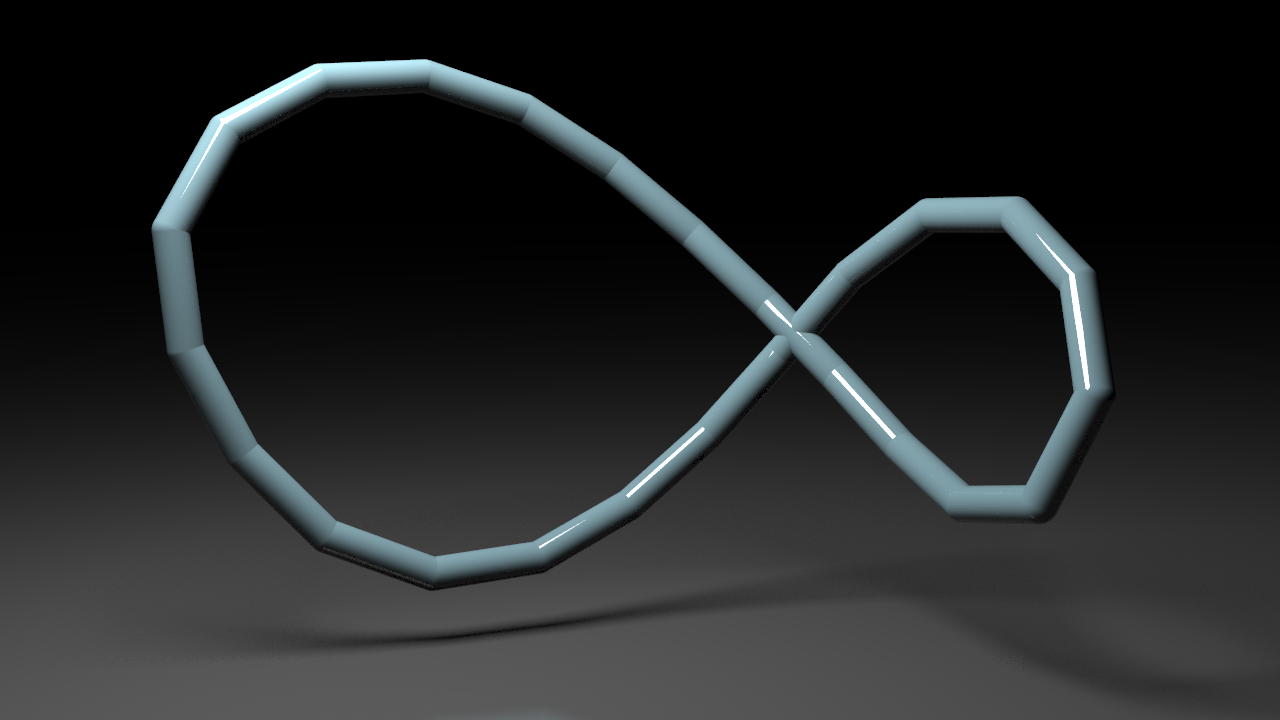
Here the corresponding parametrization using a horizontal lift
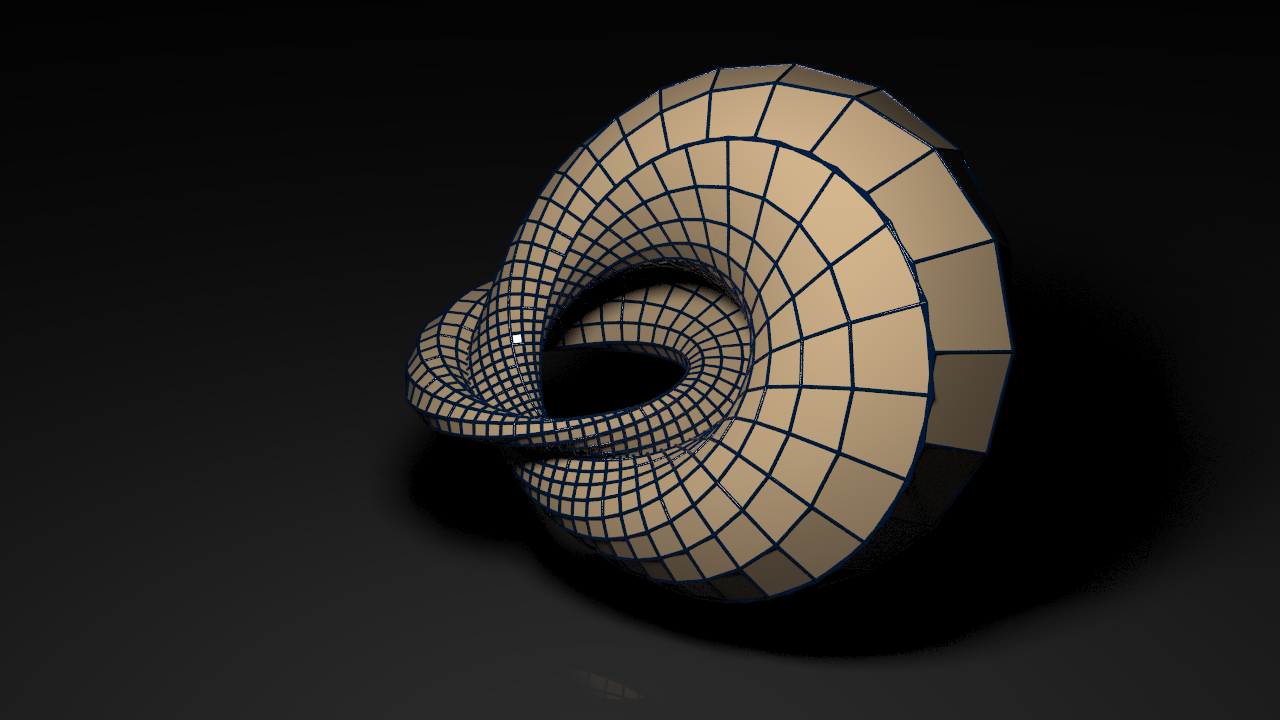
and the corresponding close-to-conformal parametrization

Just as a remark: If \(\omega \in \tfrac{1}{m}\mathbb Z\) then the grid looks already closed glueing this leads also to tori with certainly lower distortion of conformality though the underlying combinatorial torus – the mesh – is different from the standard one. Though Houdini’s fuse node can glue this. With this one gets in the end a – in a mathematical sense – very natural looking network (‘unroll’ is an ends node, ‘glue’ is a fuse node).

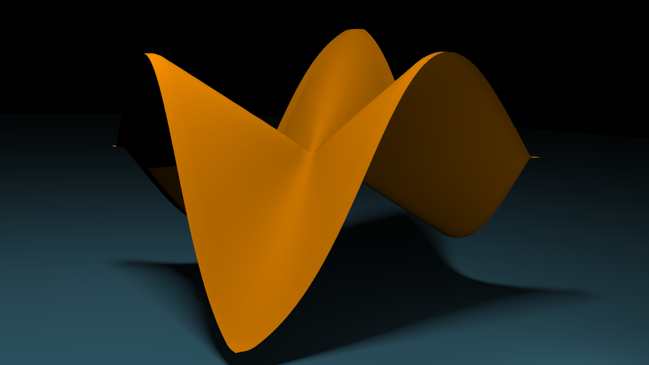
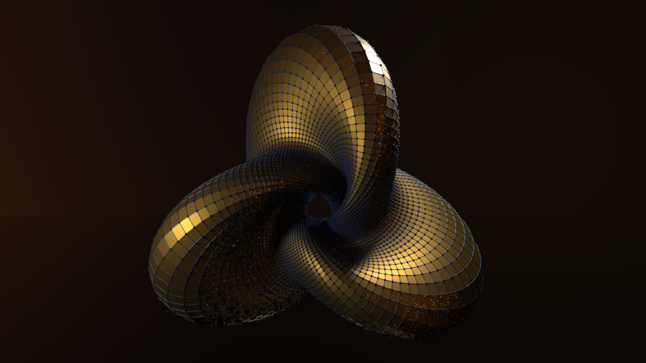
Once we have this we can ask for special curves. In “Hopf tori in \(\mathrm S^3\)” there is particular example which we can rebuild easily using a numerical trick. The curve it uses is the intersection of a cubical cone with the 2-sphere in \(\mathbb R^3\): One such cone is given by the equation\[ \tilde c (x,y,z) = x^3 + y^3 + z^3 = 0,\] i.e. it is an implicit surface and we know how we can get these in Houdini. Though in this form its symmetry axis is given by the vector \((1,1,1)\). We want the symmetry axis instead to be aligned with the \(z\)-axis. In this way we can easily stretch along the z-axis. This yields a whole 1-parameter family of curves all which enclose always an area of \(2\pi\) but have different lengths.
To change the rotation axis to \(e_3=(0,0,1)\), we can just precompose a rotation \(R\) that takes the vector \(e_3\) to the axis \((1,1,1)\). The cone is then given as the zero set of the function \[c = \tilde c \circ R.\]
To get the intersection with the round sphere we can use the cookie node. It provides the possibility to intersect two meshes (crease). If necessary one can use the join and fuse node to improve the result.

Though it may need sometimes a bit fine tuning the cookie node works quite well – as lone as the meshes are not to fine.

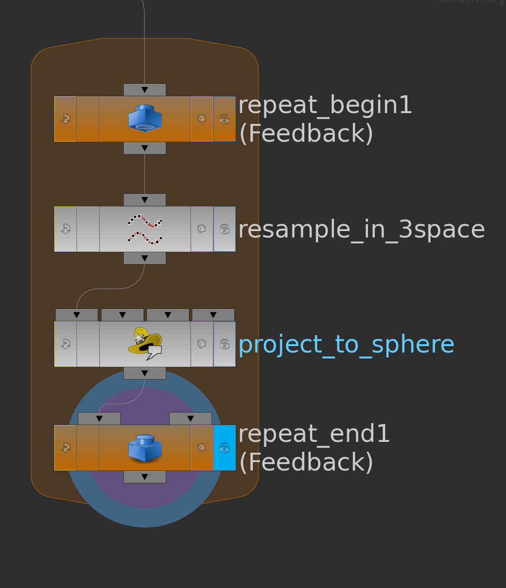
Note: The resample node will move the point of the sphere. If one wants a spherical curve with constant edge length one has to project the result back to \(\mathrm S^2\). One trick would be to iterate this. This can be done e.g. by a for-loop node.
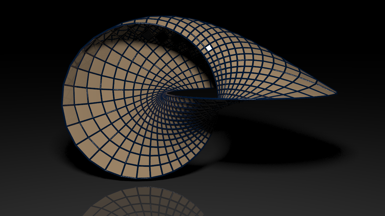
With this we can produce nice conformal parametrizations. Below a rednering of one of the tori that arise from the intersection of a cubical cone and the 2-sphere.
Homework (due 14/16 June): Write a network that creates a closed curve on \(\mathrm S^2\) and computes a parametrization of the corresponding Hopf torus. It shall be possible to switch between a horizontal and a closed lifts. Further, apply this to the intersection of the cubical cones and the 2-sphere as described above. Insert a parameter that allows to stretch along the symmetry axis.