Last time we looked at the gradient flows of functions defined on the torus \(\mathrm T^n\). This time we will look at flows on the space of Fourier polynomials \(\mathcal F_N\).
Let us first restrict ourselves to the real-valued Fourier polynomials \(\mathcal F_N^{\mathbb R} \subset \mathcal F_N\). The space \(\mathcal F_N^{\mathbb R}\) is a finite-dimensional Hilbert space and we can define the derivative of functionals and their gradient as usual: Let \(H\colon \mathcal F_N^{\mathbb R} \to \mathbb R\) be a smooth functional. Then, for \(f\in \mathcal F_N^{\mathbb R}\) and \(X\in \mathcal F_N^{\mathbb R}\),\[d_{f}H (X) =: \langle\!\langle \mathrm{grad}_f H , X\rangle\!\rangle.\]One of the most prominent functionals is the so called Dirichlet energy \(E_D\), which is defined as half the \(L^2\)-norm of the gradient: For \(f\in \mathcal F_N^{\mathbb R}\), \[E_D(f) : = \tfrac{1}{2}\int_{\mathrm T^n} |\mathrm{grad}\, f|^2 =\tfrac{1}{2}\Vert \mathrm{grad}\, f \Vert^2.\]As such the Dirichlet energy measures the ‘smoothness’ of the function. Certainly, \(E_D(f)\geq 0\) and, since \(\mathrm T^n\) is connected, we have\[f= const \Longleftrightarrow \mathrm{grad}\, f = 0 \Longleftrightarrow E_D(f) = 0.\]The Dirichlet energy is closely related to the Laplace operator \(\Delta := \mathrm{div}\circ\mathrm{grad}\).
Theorem 1. For smooth \(f,g\colon \mathrm{T^n} \to \mathbb R\), we have \(\langle\!\langle \mathrm{grad}\, f,\mathrm{grad}\, g\rangle\!\rangle = -\langle\!\langle f,\Delta g\rangle\!\rangle\).
Proof. This following from the divergence theorem and the periodicity of \(f\mathrm{grad}\, g\): From vector calculus we know that for a smooth function \(f\) and a smooth vector field \(X\) we have the following ‘product’ rule\[\mathrm{div}(fX) = \langle \mathrm{grad}\, f,X\rangle + f\mathrm{div}(X).\]Hence, with \(X= \mathrm{grad}\,g\), the divergence theorem yields\begin{align}\langle\!\langle \mathrm{grad}\, f,\mathrm{grad}\, g\rangle\!\rangle &= \int_{\mathrm{T}^n} \langle \mathrm{grad}\, f,\mathrm{grad}\, g\rangle\\ &= \int_{\mathrm{T}^n} \mathrm{div}(f\mathrm{grad}\, g) – f\mathrm{div}(\mathrm{grad}\, g) \\&= \int_{\partial \mathrm{T}^n} \langle f\mathrm{grad}\, g,N\rangle – \int_{\mathrm{T}^n}f\mathrm{div}(\mathrm{grad}\, g) \\ &= -\int_{\mathrm{T}^n} f\mathrm{div}(\mathrm{grad}\, g) \\ &= -\langle\!\langle f, \Delta g\rangle\!\rangle.\end{align}Here \(\int_{\partial \mathrm{T}^n} \langle f\mathrm{grad}\,g, N \rangle = 0\) because of the periodicity of \(f\mathrm{grad}\,g\) – the boundary integrals of opposite sides of the fundamental domain (cube) cancel. \(\square\)
Corollary 1. The Laplace operator on the torus is self-adjoint: \(\Delta^\ast = \Delta\).
Corollary 2. The gradient of the Dirichlet energy is given by \(\mathrm{grad}_f E_D= -\Delta f\).
The gradient flow of the Dirichlet energy is well-known in Physics. It is the heat equation, \[\dot f = -\mathrm{grad}_f E_D= \Delta f,\]which describes how temperature distributes in the torus.
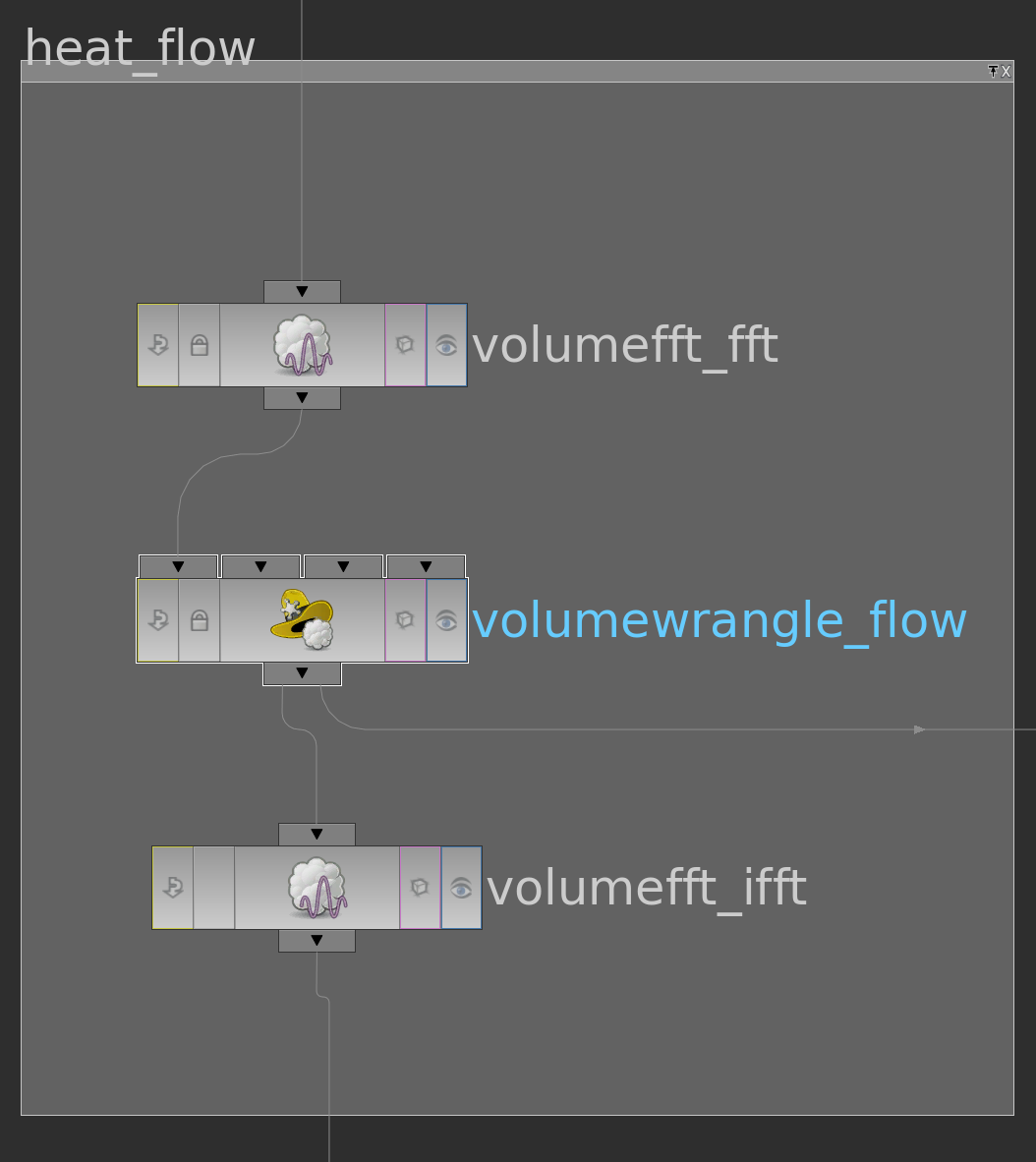
In coordinates the Laplace operator takes the usual form: If \(x_j\) denote the canonical coordinates on \(\mathbb R^n\), then\[\Delta f = \mathrm{div}(\mathrm{grad}\,f) = \sum_{i=j}^n \tfrac{\partial^2}{\partial x_j^2}f.\]Note, if \(\mathbf e_k\) is a vector of the Fourier basis, then \(\tfrac{\partial}{\partial x_j}\mathbf{e}_k = ik_j\,\mathbf{e}_k\) and hence \(\Delta \mathbf e_k = -|k|^2\mathbf e_k\). In particular the Laplacian restricts to a linear \(\mathcal F_N^{\mathbb R} \to\mathcal F_N^{\mathbb R}\) and is in fact diagonal with respect to the Fourier basis. The flow is easily computed: If \(f\in \sum_{k}c_k\mathbf e_k \mathcal F_N^{\mathbb R}\), \[\sum_k \dot c_k\mathbf e_k = \dot f = \Delta f = -\sum_k |k|^2c_k \mathbf e_k.\]Hence the coefficients solve \(\dot c_k = -|k|^2c_k\) and the flow is explicitly given as follows:\[c_k^t = e^{-|k|^2t}c_k^0.\]The heat flow is easily implemented in a small network involving two VolumeFFT nodes (for FFT and iFFT) and a VolumeWrangle node:
The VEX code is really simple:
|
1 2 3 4 5 6 7 8 9 |
float delta = chf("delta"); float m = @ix-@resx/2; float n = @iy-@resy/2; float c = exp(-(m*m + n*n)*delta); @f *= c; @g *= c; |
Here the resulting flow starting with a random function:
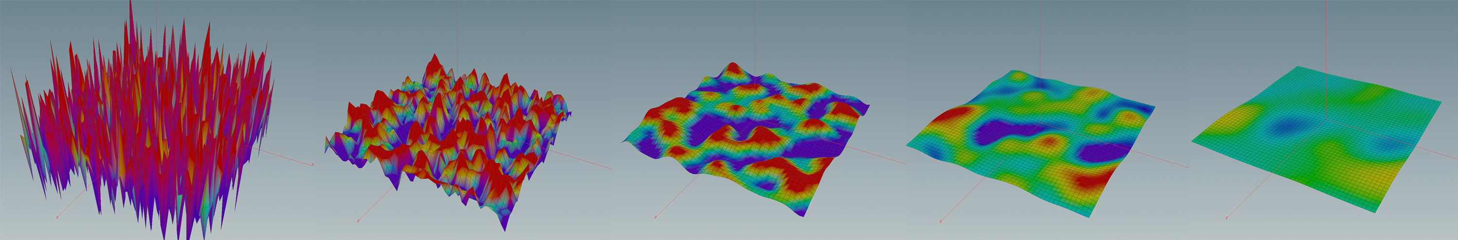
That the flow take us to the ‘constant part’ of the initial value \(f\) is obvious from the explicit form. The only coefficient that survives is \(c_0\) – this coefficient stays fixed under the flow. Moreover, \(c_0 = \langle\!\langle f, \mathbf e_0\rangle\!\rangle = \int_{\mathrm T^n} f/\int_{\mathrm{T}^n} 1 = \int_{\mathrm T^n} f/ \mathrm{vol}(\mathrm{T}^n)\). Thus, at each point \(p\in \mathrm{T}^n\), \(f_t(p)\) tends to the mean-value of \(f\) – as expected from the physical point of view. We can also look at the flow in Fourier domain (below we only show the real part). Here we see that all coefficients up to the one in the middle (corresponding to \(k=0\)) die off – the faster the higher the frequency, i.e. the further away from the center.
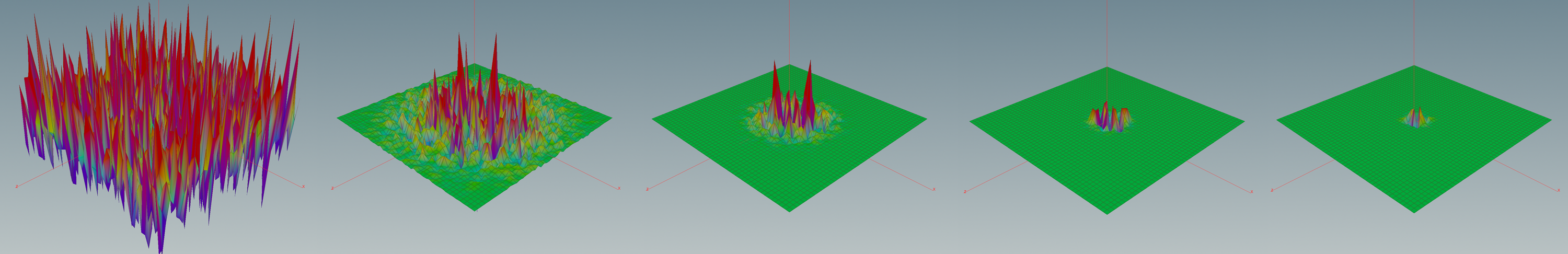
Here as we started with a random function the mean-value is expected close to zero – so seemingly nothing is left.
Now let us look at the space of complex-valued functions \(\mathcal F_N\). We can treat \(\mathcal F_N\) as a real vector space (of twice the dimension of \(\mathcal F^{\mathbb R}_N\)). The real part \(\langle\!\langle.,.\rangle\!\rangle = \mathrm{Re}\langle\!\langle.,.\rangle\!\rangle_{\mathbb C}\) of the hermitian inner product\[\langle\!\langle \psi,\phi\rangle\!\rangle_{\mathbb C} = \int_{\mathrm T^n}\overline{\psi}\phi, \quad \psi,\phi\in\mathcal F_N,\]turns \(\mathcal F_N\) into a Euclidean vector space and we can define the gradient of a smooth functional \(H\colon \mathcal F_N \to \mathbb R\) as before.
Note that if \(\psi = f+ig\) and \(\phi = u+iv\), then \(f,g,u,v \in \mathcal F_N^{\mathbb R}\) and we have\[\langle\!\langle \psi,\phi\rangle\!\rangle = \mathrm{Re}\int_{\mathrm T^n}\overline{\psi}\phi = \int_{\mathrm T^n}\mathrm{Re}\bigl((f-ig)(u+iv)\bigr) = \int_{\mathrm T^n} (fu+gv) = \langle\!\langle f,u\rangle\!\rangle + \langle\!\langle g, v\rangle\!\rangle.\]Further \(\Delta \phi = \Delta u + i\Delta v\) and thus \(\langle\!\langle \psi,\Delta \phi\rangle\!\rangle = \langle\!\langle f,\Delta u\rangle\!\rangle + \langle\!\langle g, \Delta v\rangle\!\rangle\). Hence we also have in the complex-valued case that\[\mathrm{grad}_\psi E_D = -\Delta \psi.\]Moreover, the imaginary part of the hermitian inner product yields a non-degenerate skew-symmetric bilinear form \(\sigma\) – a symplectic form,\[\sigma(X,Y) = \mathrm{Im}\langle\!\langle X, Y\rangle\!\rangle,\]which we can use to define a symplectic gradient. Certainly, the symplectic forms \(\sigma\) and the real inner product \(\langle\!\langle .,.\rangle\!\rangle\) satisfy the following relation:\[\sigma(X,Y) = \langle\!\langle i X, Y\rangle\!\rangle.\]Thus, for any smooth functional \(H\colon \mathcal F_N \to \mathbb R\), we have\[\mathrm{sgrad}_{\psi} H = -i\,\mathrm{grad}_\psi H .\]One easily shows the following theorem.
Theorem 2. If \(\gamma\) is an integral curve of \(\mathrm{sgrad}\,H\), then \(H\circ\gamma = const\).
Proof. We just have to differentiate \(H\circ \gamma\):\[\frac{d}{dt} (H\circ\gamma) = d_\gamma H(\frac{d}{dt}\gamma) = d_\gamma H(\mathrm{sgrad}_\gamma H) = -\langle\!\langle \mathrm{grad}_{\gamma}H,i\mathrm{grad}_\gamma H\rangle\!\rangle = 0.\]Thus \(H\circ\gamma\) is constant. \(\square\)
The flow of \(\mathrm{sgrad}\,E_D\) preserves the Dirichlet energy and is well-known in Physics: Actually, \(\dot\psi = \mathrm{sgrad}_\psi E_D\) is the famous (linear) Schrödinger equation\[i\dot\psi = \Delta \psi,\]which plays an important role in quantum mechanics. Again we can easily solve this equation in Fourier domain: The flow on the coefficients is given by\[c_k^t = e^{i|k|^2t}c_k^0.\]The network looks as for the heat equation – only the VEX code changes slightly:
|
1 2 3 4 5 6 7 8 9 10 11 12 13 |
float delta = chf("delta"); float m = @ix-@resx/2; float n = @iy-@resy/2; float c = cos((m*m + n*n)*delta); float s = sin((m*m + n*n)*delta); float a = @f; float b = @g; @f = c*a - s*b; @g = c*b + s*a; |
Since we are dealing with complex-valued functions now, we need to come up with a way to visualize them. One common way to do this is to visualize the magnitude of the complex number as graph and the phase by colors. Therefore one has to come up with a suitable (periodic) color map. To set the colors we can directly set the @Cg-attribute using a PointWrangle node. Here is one possible choice (@phase denotes the argument of the complex value and was computed in a previous node):
|
1 |
@Cd = set(cos(@phase+PI)/2+0.5,sin(@phase)/2+.5,1); |
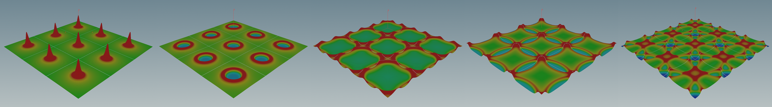
Starting with a peak centered at \(0\) the flow looks as follows:
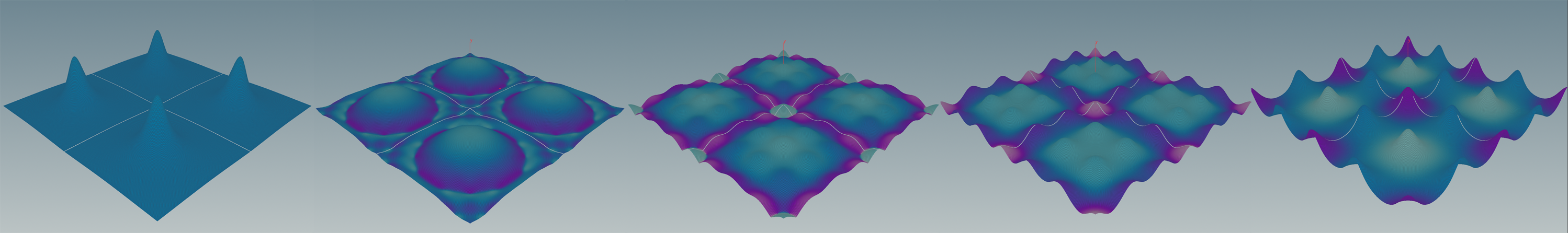
Actually, this reminds to waves. Let us again restrict to real-valued functions. The wave equation can be treated easily within our setup – it is an equation of second order: \[\ddot f = \Delta f.\]By what we have seen already it is clear how this translates to the coefficients \(c_k\) of the Fourier polynomial:\[\ddot c_k = -|k|^2 c_k.\]To solve this equation of second order we can translate it to an equation of first order: If\[\begin{pmatrix}u\\v\end{pmatrix}^{\Large\cdot} =\begin{pmatrix}0 & 1\\ -|k|^2 & 0\end{pmatrix}\begin{pmatrix}u\\v\end{pmatrix},\]then\[\ddot u = \dot v = -|k|^2 u.\]In general, consider the linear differential equation \(\dot x = Ax\) for \(A\in \mathbb R^{m\times m}\). Let \(v\) be an eigenvector of \(A\) with eigenvalue \(\lambda\). Then \(\gamma(t) = e^{t\lambda} v\) is an integral curve:\[\gamma^\prime(t) = \lambda e^{t\lambda } v =e^{t\lambda} Av = A \gamma(t).\]Thus, if \(\{v_1,…,v_m\}\) is a basis of eigenvectors and \(\lambda_1,…,\lambda_m\) denote the corresponding eigenvalues, then the flow is given by\[\Phi(t,x_0) = B \begin{pmatrix}e^{t\lambda_1} & & 0 \\ & \ddots & \\ 0 & & e^{t\lambda_m} \end{pmatrix}B^{-1}x_0,\quad B= (v_1,…,v_m).\]The eigenvalues of our \(2\times 2\) mini system are obviously \(\pm i|k|\) and the corresponding eigenvectors are \[v_{\pm} = \begin{pmatrix}1 \\ \pm i|k|\end{pmatrix}.\]Thus, if we restrict ourselves to initial velocity \(\dot u (0) = v(0) = 0\), then we get that \(u\) is of the form \[u(t) = const\cdot (e^{i|k|t} + e^{-i|k|t}) = const\cdot \cos (|k|t).\]Hence we find that the solution of the wave equation is given by\[c_k^t = \cos(|k|t)c_k^0.\]If we let this start with an initial peak then the result looks as follows (here we are dealing with real-valued functions again – as in the heat flow pictures the color encodes the value of the real function):
Homework (due 28/30 June). Write a network that computes to a given discrete function \(f\) the solutions of the heat, the Schrödinger and the wave equation with initial condition \(f\). Try several initial condition.