
In the last post we created geometric objects from scratch, including the underlying combinatorics. In most situations it is much more convenient to start with already existing geometry and transform it.
This approach is similar to the standard way of dealing with curves and surfaces in Differential Geometry: One starts with a parameter domain $M$ which could be a subset of $\mathbb{R}^n$ or just an abstract $n$-dimensional manifold. For concreteness, just imagine that $n$ is either one (for the study of curves) or two (for surfaces). The geometric objects of interest are then certain smooth maps $f:M \to \mathbb{R}^3$. Such an $f$ is then called a parametrized curve (in case $n=1$) or a parametrized surface (if $n=2$).
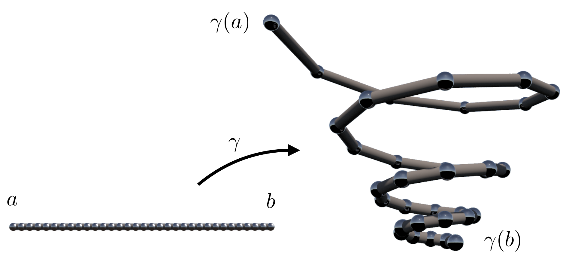
If $M$ is a compact connected one-dimensional manifold with non-empty boundary we can as well assume that $M$ is a closed interval $[a,b]$ on the real line:
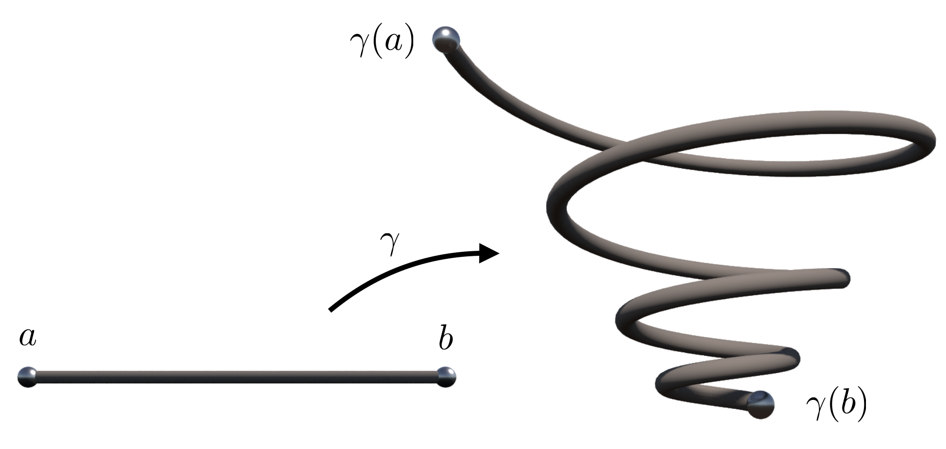
In Houdini a discrete version of the interval $[a,b]$ can conveniently supplied by a Grid node where the Rows has been set to one. The Columns parameter specifies the number of equally spaced sample points on interval. Instead of specifying $a,b$ directly we have to provide $b-a$ as the first component of the Size parameter and $(a+b)/2$ as the first component of the Center parameter. Afterwards we use a node of type Point Wrangle in order to map the $x$-coordinate to the desired space curve. The curve in the last picture results from the VEX code below. alpha, omega and lambda are three float parameters of that Point Wrangle node.
|
1 2 3 4 5 6 7 8 9 10 11 12 13 |
#include "Math.h" float alpha = PI/180 * ch("alpha"); float omega = ch("omega"); float lambda = ch("lambda"); float t = @P.x; float c = cos(alpha); float s = sin(alpha); float r = exp(lambda * t); @P.z = r * s * cos(omega * t); @P.x = r * s * sin(omega * t); @P.y = r * c; |
If $M$ is a compact connected one-dimensional manifold without boundary then we can as well assume that $M$ is the unit circle $S^1\subset \mathbb{R}^2$:
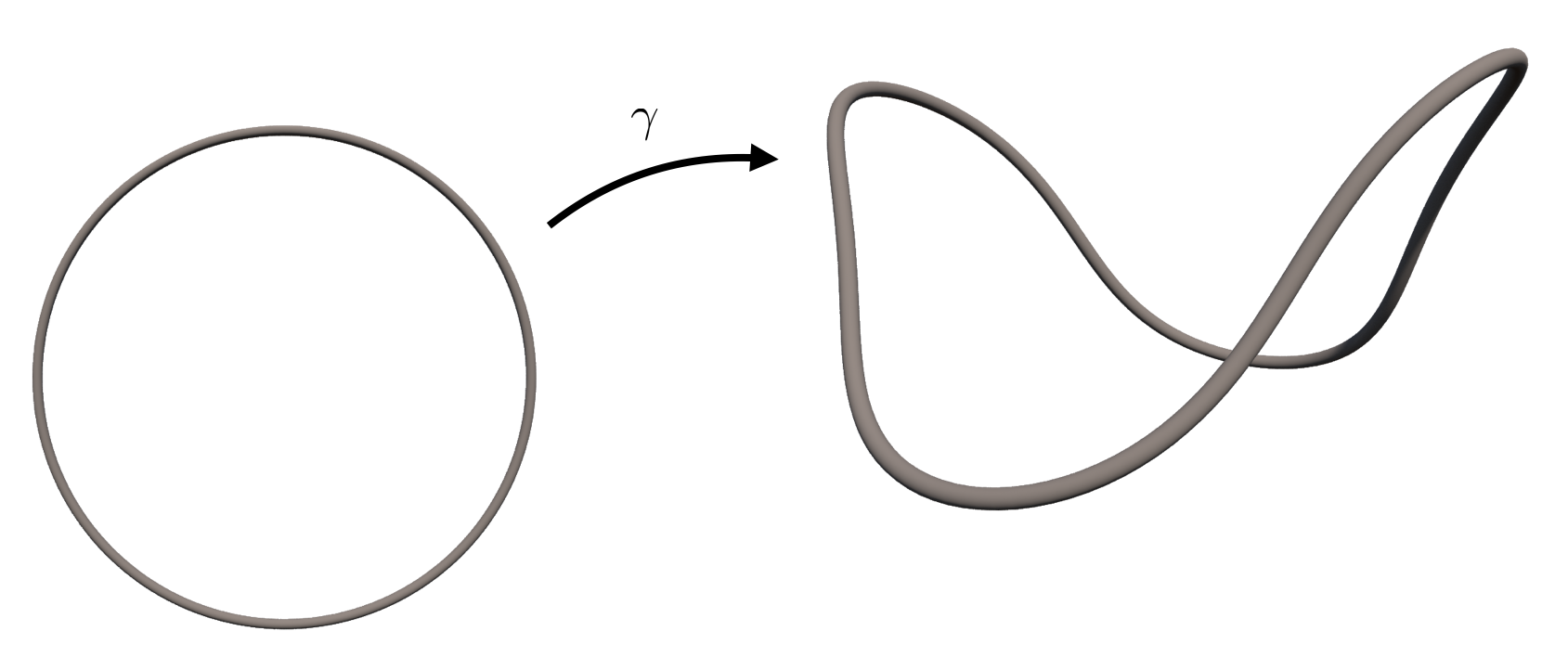
In Houdini a discrete version of the unit circle $S^1$ can conveniently supplied by a Circle node where the Primitive Type has been set to Polygon. The Divisions parameter specifies the number of equally spaced sample points on the circle. Afterwards we use a node of type Point Wrangle in order to map the$(x,y)$-coordinates on the circle to the desired space curve. The curve in the last picture results from the VEX code below. k is an integer parameter and r a float parameter of that Point Wrangle node.
|
1 2 3 4 5 6 7 8 9 10 11 12 13 14 15 16 17 18 |
#include "math.h" #include "$HIP/include/Complex.h" float k = ch("k"); float r = ch("r"); float q = pow(r,2*k-1); float m = 2*k-1; float a = 1/(2*k-1); float b = 2*pow(r,k)/k; float fac = 1/(r+q); float c = @P.x; float s = @P.y; vector2 zm = cpow(set(c,s),(int)m); vector2 zk = cpow(set(c,s),(int)k); @P.x = fac*(r*c + a*q*zm.x); @P.y = fac*b*zk.y; @P.z = fac*(r*s - a*q*zm.y); |
We have used here an include file which implements some complex arithmetic.
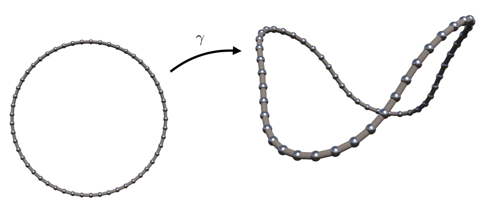
Note that the sample points on the space curve roughly look equally spaced. The reason is that in this particular example the corresponding smooth curve is parametrized by arclength for all values of the parameters $k,r$. We leave the proof of this fact as an exercise. This means that if $p$ runs through the unit circle with unit speed then also $\gamma(s)$ travels with unit speed.