
Let $\Omega \subset \mathbb{R}^n$ be a domain, we will consider $\Omega$ to be the “space” and functions:
\begin{align}
f : \mathbb{R} \times \Omega \rightarrow \mathbb{R}, \\ (t,x) \mapsto f(t,x),\end{align}
will be view as time dependent functions
\begin{align}
& f_t : \Omega \rightarrow \mathbb{R}, \\ & f_t(x) := f(t,x).\end{align}
We want to investigate partial differential equations (PDE’s) for $f$, that involve the Laplace operator. Here the Laplace operator is defined just for the space coordinates $x$:
\[\left(\Delta f\right) (t,x) := \left(\Delta f_t\right) (x) := \sum_{i=1}^n \frac{\partial^2 f_t(x)}{\partial x_i^2}.\]
Typical examples for such PDE’s from physics are:
- Wave equation: \[\frac{\partial^2 f}{\partial t^2} = c^2 \Delta f, \quad \quad \quad c \in \mathbb{R}.\]
- Heat equations: \[\frac{\partial f}{\partial t} = c \Delta f, \quad \quad \quad c \in \mathbb{R}.\]
We will investigate these PDS’s on closed triangulated surfaces $\Omega = M = (V,E,F)$, where we only have finitely many function values i.e. :
\begin{align} & f : \mathbb{R} \rightarrow \mathbb{R}^V, \\& f(t) = \left( \begin{matrix} f_1(t) \\ \vdots \\ f_N(t) \end{matrix} \right) .\end{align}
On $M$ we have the usual Laplace operator $\Delta :\mathbb{R}^V \rightarrow \mathbb{R}^V$ and for the above PDE’s we obtain ordinary differential equations (ODE’s):
- Wave equation: \[\ddot{f}(t)= c^2 \Delta f(t).\]
- Heat equations: \[\dot{f}(t)= c \Delta f(t).\]
This is a big improvement since it is fare more complicated to solve PDE’s then ODE’s.
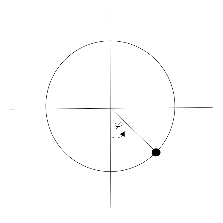
Before we will present some methods to solve ODE’S numerically consider the Pendulum equation as example:
\[\ddot{\varphi} = -\sin(\varphi).\]
The standard procedure to solve a second order ODE is to transfer it in a system of two ODE’s of first order. Therefore consider:
\begin{align} & f : \mathbb{R} \rightarrow \mathbb{R}^2, \\& f(t) = \left( \begin{matrix} \varphi (t) \\ \dot{\varphi} (t) \end{matrix} \right) .\end{align}
Then $\varphi$ solves the pendulum equation if and only if $f$ solves
\[\left( \begin{matrix} u \\ v \end{matrix} \right)^{\bullet} = \left( \begin{matrix} v \\ -\sin (u) \end{matrix} \right). \]
The energy of the above system is given by $E(t) := \frac{1}{2}\dot{\varphi}^2 – \cos(\varphi).$ $E$ is a constant of motion since:
\[\dot{E} = \dot{\varphi} \ddot{\varphi} + \dot{\varphi} \sin (\varphi) = o,\]
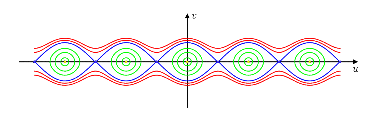
The level-sets of the energy of the pendulum. The yellow dots correspond to $E=-1$, the green curves to $-1<E<1$, the blue ones to $E=1$ and the red ones to $E>1$.
if $\varphi$ is a solution of the pendulum equation. In the phase space the solutions of the ODE are implicitly given by the level-sets of $E$ :
By the theorem of Picard-Lindelöf there is for every $\left( \begin{matrix} u_0 \\v_0 \end{matrix} \right) \in \mathbb{R}^2 $ a unique solution of the initial value problem (IVP) :
\begin{align} & \left( \begin{matrix} u \\ v \end{matrix} \right)^{\bullet} = X(u,v) = \left( \begin{matrix} v \\ -\sin (u) \end{matrix} \right) \\ & \left( \begin{matrix} u \\ v \end{matrix}\right)(0) = \left( \begin{matrix} u_0 \\ v_0 \end{matrix} \right).\end{align}
These solutions lie on the level-sets of $E$.
Now we want to approximate the solution of the IVP by a sequence
\[\ldots,\left( \begin{matrix} u_{-1} \\ v_{-1} \end{matrix} \right), \left( \begin{matrix} u_0 \\ v_0 \end{matrix}\right) , \left( \begin{matrix} u_1 \\ v_1 \end{matrix} \right),\ldots \in \mathbb{R}^2\]
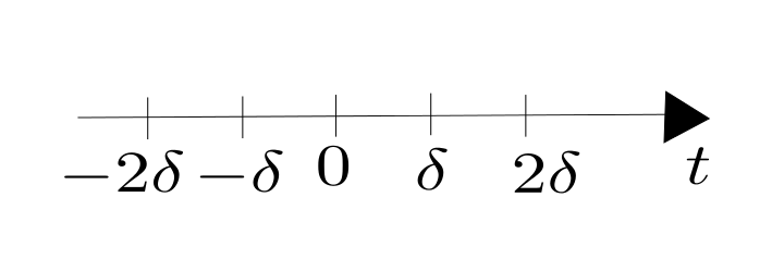
such that for the real solution $\left( \begin{matrix} u(t) \\ v(t) \end{matrix} \right)$ we have $\underbrace{\left( \begin{matrix} u_k \\ v_k \end{matrix} \right)}_{p_k} \approx \left( \begin{matrix} u \\ v\end{matrix} \right) (k\delta), $
where $\delta$ is the time step.
There are several methods to get such a sequence:
1. Forward Euler method:
Let $ X: \mathbb{R}^2 \rightarrow \mathbb{R}^2$ be the vectorfiled representing the ODE , i.e. \[\left( \begin{matrix} u \\ v \end{matrix} \right)^{\bullet} (k\delta)= X(u(k\delta),v(k\delta)) = X(p_k).\]
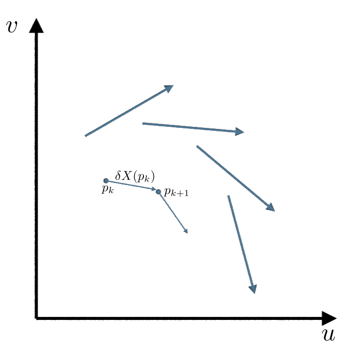
Then with the forward Euler method we get from $p_k$ to $p_{k+1}$ by walking for the time $\delta$ in the direction of $ X(p_k)$.
\[p_{k+1} = p_k + \delta X(p_k).\]
The big advantage of this method is, that it is very fast. The disadvantage is illustrated in the following example: For the harmonic oscillator the ODE is given by the vectorfield:
\[X(u,v) = \left( \begin{matrix} v \\ -u \end{matrix}\right).\]
Its analytic solution is:
\[ \left( \begin{matrix} u \\ v \end{matrix}\right)(t) = \left( \begin{matrix} \cos(t) & \sin(t)\\ -\sin(t) & \cos(t)\end{matrix}\right) \left( \begin{matrix} u_o \\ v_0\end{matrix}\right)\]
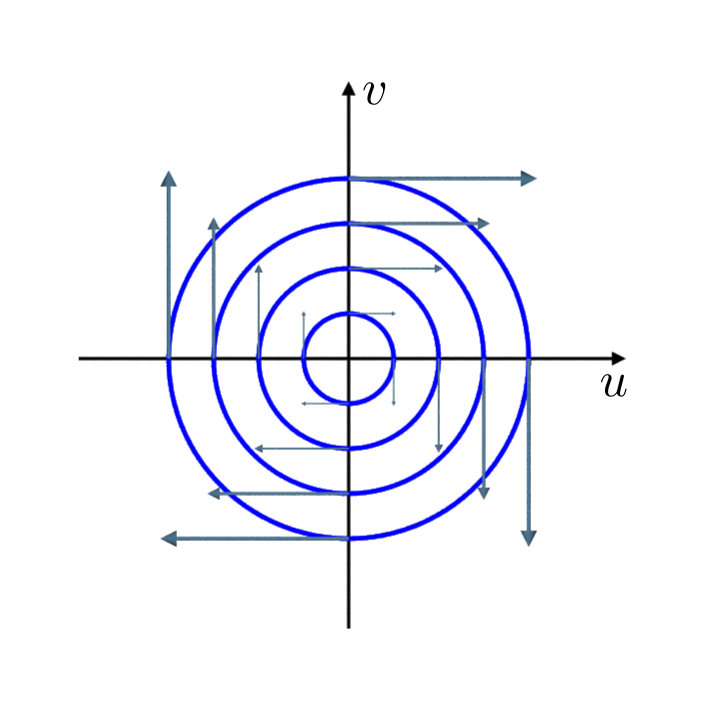
The vector field and the corresponding integralcurves of the harmonic oscillator.
The energy is a again a constant of motion: $E(t) := \frac{1}{2} \left( u^2 + v^2 \right)$ and the level-sets of $E$ are circles. If we apply the forward Euler method the solution is a spiral and not a circle. Therefore, the energy gets bigger and bigger and the solution blows up.
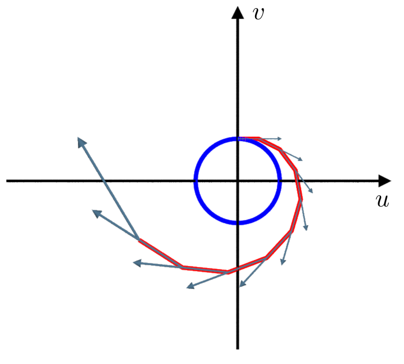
The real integralcurve (blue) and the one obtain with the Euler forward method for $\delta = 0.5$ (red), together with the corresponding vectorfield (grey).
2. Backward Euler method:
The backward Euler method works in the following way: Find $p_{k+1}$ such that one Euler forward step with respect to the vectorfield $-X$ gives you $p_k$. i.e
\[p_k = p_{k+1} -\delta X(p_{k+1}).\]
That means we have to solve the following non linear system of equations to get from $p_k$ to $p_{k+1}$:
\[p_{k+1} = p_k + \delta X(p_{k+1}).\]
This can for example be done with the classical Newton method. The advantage of the backward Euler method is that the energy does not increase and therefore the solution does not blow up. The disadvantage is that solving a non linear system of equations can be hard and expensive.
The idea behind both Euler methods, that guaranties the convergence to the real solution for $\delta \rightarrow 0$ is given by the mean value theorem: For $f \in C^1(\mathbb{R},\mathbb{R}^n)$, $p \in \mathbb{R}$ and $\delta >0$ there exist $\tau \in (p,p+\delta)$ such that”
\[f'(\tau) = \frac{f(p)-f(p+\delta)}{\delta}.\]
3. Verlet method:
The Verlet method works for equations of the form \[\ddot{f}(t) = F\left( f(t)\right), \quad \quad \quad \quad \quad f \in C^2(\mathbb{R},\mathbb{R}^n).\]
In order to approximate $f(k\delta)$ by $p_k$ we use the mean value theorem twice:
\begin{align}\ddot{f}(t) & \approx \frac{\dot{f}\left(t+\frac{\delta}{2}\right) -\dot{f}\left(t-\frac{\delta}{2}\right)}{\delta} \approx \frac{\frac{f \left( t+\delta\right) -f \left(t\right) }{\delta} -\frac{ f \left( t\right) -f \left( t-\delta\right) }{\delta}}{\delta}\\ & = \frac{f( t + \delta) -2f(t) + f(t-\delta)}{\delta^2}.\end{align}
This gives us the following recursion formula for the $p_k$’s:
\begin{align} F(p_k) & = \frac{p_{k-1} -2p_k + p_{k+1}}{\delta^2}\\ \Leftrightarrow \quad p_{k+1} & = 2p_k -p_{k-1} + \delta^2 F(p_k).\end{align}
To solve this recursion formula, we start with the initial data \[ \left( \begin{matrix} p_0 \\ p_1 \end{matrix} \right) := \left( \begin{matrix} u_0 \\ v_1 \end{matrix} \right) := \left( \begin{matrix} f(0) \\ f(\delta) \end{matrix} \right) \]
with the approximation:
\begin{align} \frac{p_0 + p_1}{2} \approx f\left( \frac{\delta}{2}\right), \\ \frac{p_1-p_0}{\delta} \approx \dot{f}\left( \frac{\delta}{2}\right), \end{align}
this corresponds to the usual initial data of an IVP for a for a second order ODE. Afterwords we use:
\[\left( \begin{matrix} p_k \\ p_{k+1} \end{matrix} \right) = \left( \begin{matrix} u_k \\ v_k \end{matrix} \right) = \left( \begin{matrix} v_{k-1} \\ 2v_{k-1} -u_{k-1} + \delta^2 F(v_{k-1}) \end{matrix} \right) . \]
If we consider that as a two dimensional system with $q_k := \left( \begin{matrix} u_k \\ v_k \end{matrix} \right)$, we have:
\[q_{k+1} = X(q_k) ,\]
with:
\begin{align} & X:\mathbb{R}^2 \rightarrow \mathbb{R}^2, \\ & X(u,v) = \left( \begin{matrix} v \\ 2v -u + \delta^2 F(u) \end{matrix} \right). \end{align}
This is a very good choice of discretization, because the vectorfield $X$ is area preserving:
\[X'(u,v) = \left( \begin{matrix} 0 & 1 \\ -1 & 2 + \delta^2 F'(u) \end{matrix} \right) \leadsto \det X'(u,v) = 1.\]
This gives us for $U \subset \mathbb{R}^2:$
\[\mbox{area}\left(X(U)\right) = \int_{X(U)} 1 = \int_U |\det X’ (u,v)| = \int_U 1 = \mbox{area}(U).\]
There is a huge theory about area preserving maps and their higher dimensional analog symplectic maps. This maps lead to so called symplectic integrators, that do an excellent job solving ODE’s.
Lets get back to the pendulum equation: $\ddot{\varphi} = -\sin(\varphi).$ If we use a clever method for the discretization of $F(\varphi) = \sin(\varphi)$, the Verlet method gives us a good solution of the pendulum equation.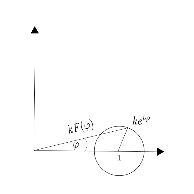 Where the clever discretization of $F$ is the following: \[F(\varphi) = \frac{1}{k}\arg \left( 1 + k e^{i\varphi} \right).\]