
In class we discussed how to generate smoothed random functions on the discrete torus and how to compute their discrete gradient and the symplectic gradient. In this tutorial we want to visualize the corresponding flow.
As described in a previous post, the inverse of the sampling operator provides an identification between functions on the discrete torus \(\mathrm T_d^2= \mathbb Z^2/(2N+1)\mathbb Z^2\) and the Fourier polynomials \(\mathcal F_N\) on the torus \(\mathrm T^2 = \mathbb R^2/2\pi\mathbb Z^2\): If \(f\colon\mathrm T_d^2 \to \mathbb R\subset \mathbb C\), then the corresponding Fourier polynomial is given by\[\hat f = \sum_k c_k \mathbf e_k ,\]where the coefficients are given by the FFT of the discrete function \(f\) and the index \(k\) runs over the grid points \(k\) of the discrete torus (i.e. all \(k\) with \(\mathrm{max}\,|k_j|\leq N\)). Let us call the map that sends a discrete \(f\) to the polynomial \(\hat f\) by \(F\).
Since the Fourier polynomials are smooth functions, \(F\) provides a way to define a discrete gradient: If \(g\) is a smooth function defined on an open \(U\subset \mathbb R^2\), then the gradient \(\mathrm{grad}\, g \colon U \to \mathbb R^2\) of \(g\) is defined by\[d_p g(X) = \langle \mathrm{grad}_p g, X\rangle.\]Here \(\langle.,.\rangle\) denotes the Euclidean inner product. If \(\frac{\partial}{\partial x_j}\) denotes the partial derivative with respect to the \(j\)-th coordinate of \(\mathbb R^2\). Then we find that\[\mathrm{grad}\, g = \begin{pmatrix}\frac{\partial g}{\partial x_1} \\\frac{\partial g}{\partial x_2}\end{pmatrix}.\]Using \(F\) we then get a discrete partial derivates \(\frac{\tilde\partial}{\partial x_j}\) as follows:\[\frac{\widetilde\partial}{\partial x_j} : = F^{-1}\circ\frac{\partial}{\partial x_j}\circ F.\]More explicitly, since \(\mathbf e_k(x) = \tfrac{1}{2\pi}e^{i\langle k,x\rangle}\), we have \(\tfrac{\partial}{\partial x_j}\mathbf e_k = i\,k_j\,\mathbf e_k\). Thus, for a Fourier polynomial \(\hat f = F(f) = \sum_{k}c_k\mathbf e_k\), we get\[\frac{\widetilde\partial}{\partial x_j}f = F^{-1}\Bigl(\frac{\partial \hat f}{\partial x_j}\Bigr) = F^{-1}\Bigl(\sum_k c_k\frac{\partial \mathbf e_k}{\partial x_j}\Bigr) =F^{-1}\Bigl(\sum_k i\, k_j \,c_k \mathbf e_k\Bigr).\]With this we can define the gradient of discrete function \(f\colon \mathrm T^2_d \to \mathbb R\) in analogy to the smooth case:\[\mathrm{grad}\, f = \begin{pmatrix}\frac{\widetilde\partial}{\partial x_1}f \\\frac{\widetilde\partial}{\partial x_2}f\end{pmatrix}.\]So let us pick a discrete random function smooth it using a periodic blur. As explained in a previous post a random function can be created with help of erf_inv. Since uniformly distributed points in \([0,1]\) are provided by the rand method of VEX, this is simple to implement: For each point of the 2d-volume we pick a uniformly distributed value x in \([0,1]\). Then f = erf_inv(2 x -1) will be a random function. Here an example network and the corresponding result:
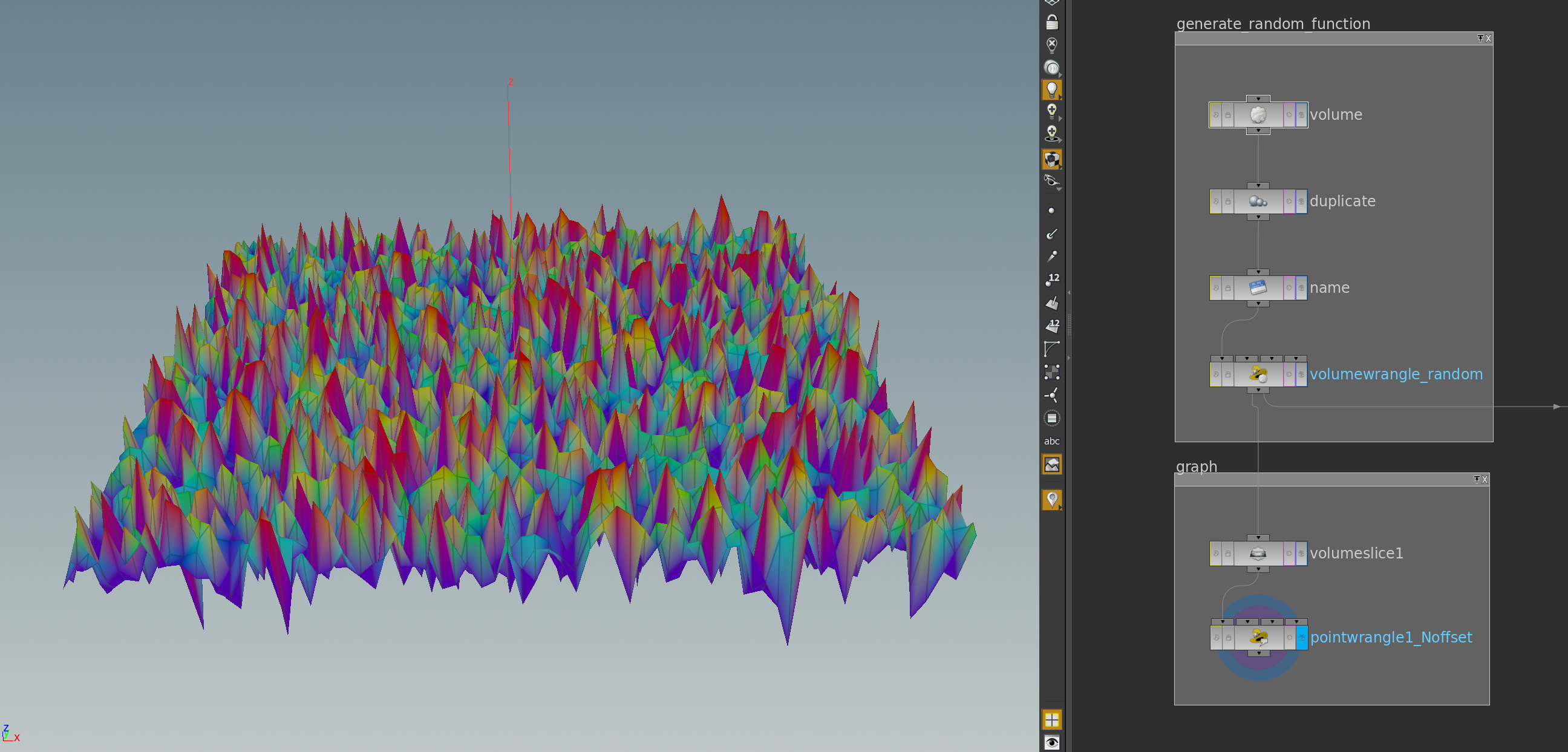
The graph is made by a volume slice node colored by the function values followed by a point wrangle node shifts the point positions in the normal direction (attribute @N). Here the two lines VEX code that generate the random function:
|
1 2 |
vector4 seed = set(@P.x,@P.y,@P.z,1); @f = erf_inv(2*rand(seed)-1); |
Note that the rand method needs a seed which we choose here to be the vector4 that contains the coordinates supplemented with an integer. Though not crucial here this is a possibility to generate several different random function (a different integer for each random function).
To smooth this random function we can write a blur node that takes into account that we are actually dealing with periodic functions. This way we get a smoothed version of the random function \(f\). Below the network
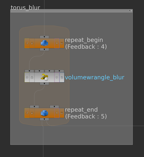
and the code for the volume wrangle
|
1 2 3 4 5 6 7 8 9 10 11 12 13 14 15 16 17 18 19 20 21 |
vector r =chv("r"); int rx = (int)r.x; int ry = (int)r.y; int rz = (int)r.z; float a=0; float b=0; for (int dx=-rx; dx<rx+1; dx++) { for (int dy=-ry; dy<ry+1; dy++) { for (int dz=-rz; dz<rz+1; dz++) { int jx = (@ix+dx) % @resx; int jy = (@iy+dy) % @resy; int jz = (@iz+dz) % @resz; a += volumeindex(0,"f",set(jx,jy,jz)); b += volumeindex(0,"g",set(jx,jy,jz)); } } } float fac = (2*rx+1)*(2*ry+1)*(2*rz+1); @f = a/fac; |
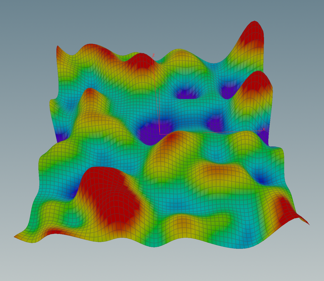
Here r is referring to a parameter of the node that specifies the number of points to average over in the x-, y- and z-direction. After the blur the function will look similar to this one:
Now that we have our discrete function \(f\) we want to compute its gradient. Therefore we transform \(f\) in the Fourier domain using the Volume FFT node provided by Houdini.
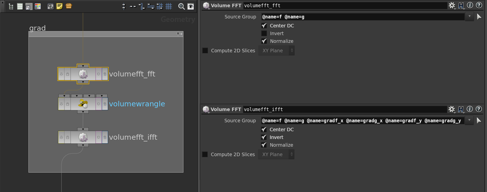
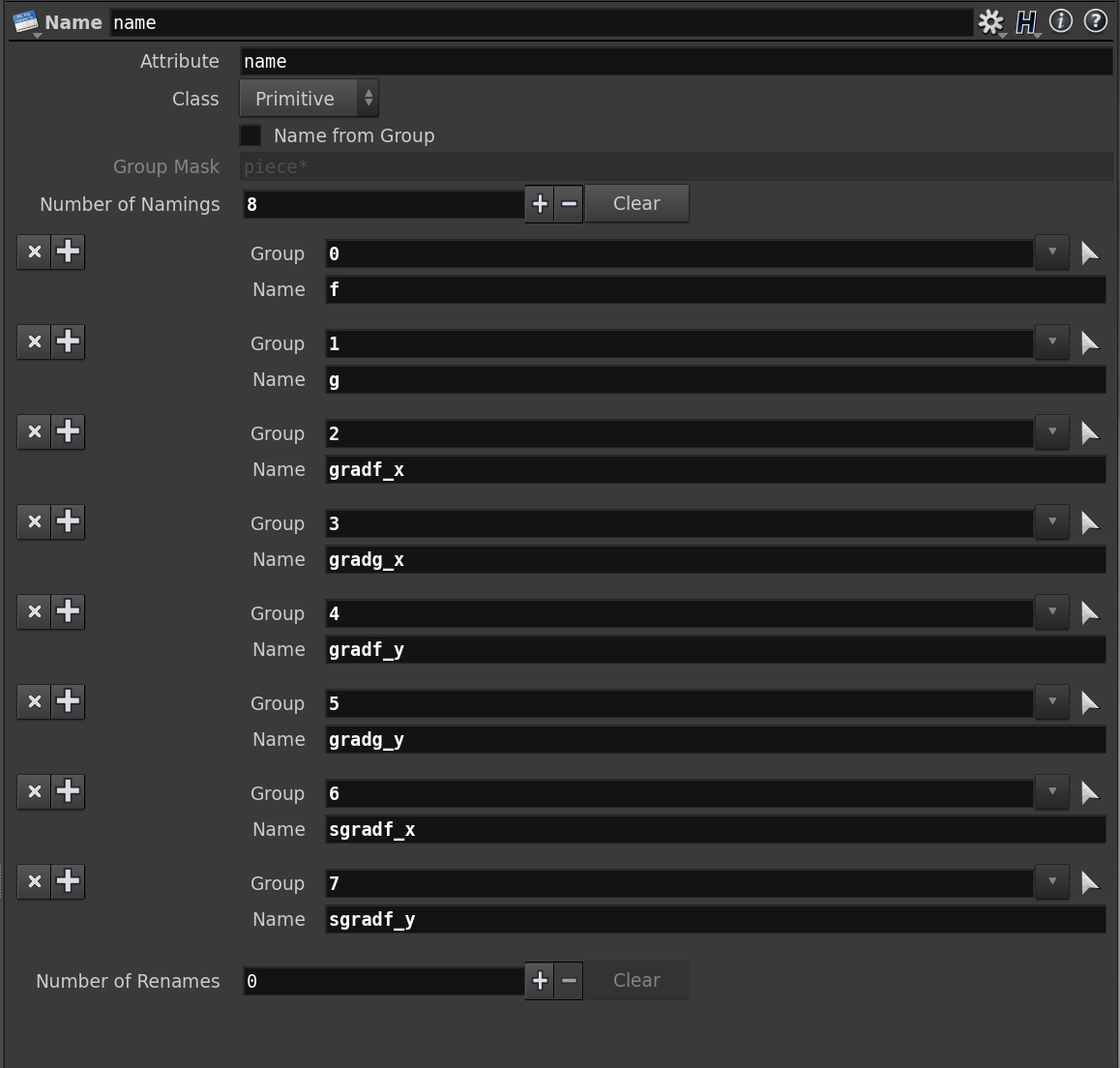
Note that we used the center option here which shifts the grid point \((0,0)\) to the middle of the volume. Note also that we hand over a second function \(g\) to the FFT node which represents the imaginary part of our discrete function, i.e. \(g=0\). So we only need to instantiate \(g\) and leave it then as it is. We also need later a volumes that store the components of \(\mathrm{grad}\, f\). Therefore, right at the beginning, we duplicate the volume as often as we need it and name the copies then afterwards (compare with the part of the network that generates the random function).
After the FFT node the coefficients of the Fourier polynomial \(\hat f\) are stored in \(f\) and \(g\) (with a shift by in \(x\) and \(y\) direction). We then compute the partial derivatives in Fourier domain in a volume wrangle node. The corresponding VEX code is shown below.
|
1 2 3 4 5 6 7 8 |
float m = @ix-@resx/2; float n = @iy-@resy/2; @gradf_x = -m * @g; @gradg_x = m * @f; @gradf_y = -n * @g; @gradg_y = n * @f; |
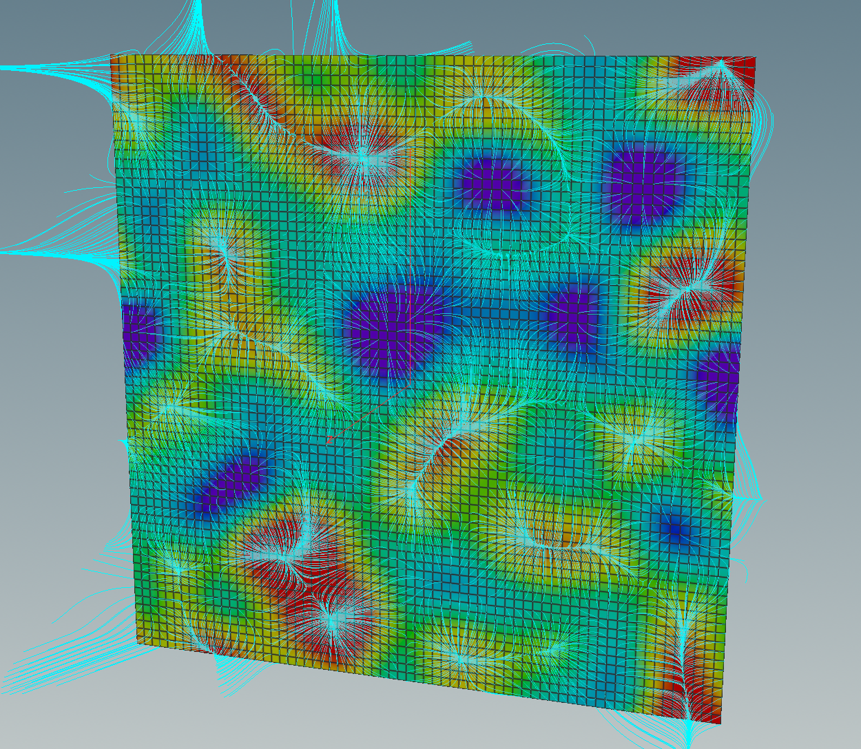
After that we can transform everything back to the spatial domain using the FFT node again – this time with the inverse button selected. The outcome is a vector field which can be visualized by a volume slice node followed by a volume trail node. We merge that with another volume slice to display \(f\). Here the network
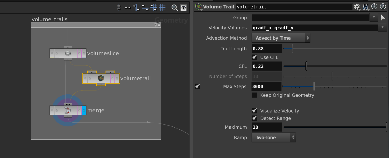
and the resulting picture of the integral curves
Let us shortly switch back to the smooth setup. On \(\mathbb R^2\) we have a second bilinear form:\[\sigma(X,Y) := \det (X,Y).\]
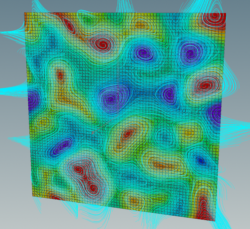
This form can be used to define another vector fields out of the differential \(df\): The symplectic gradient \(\mathrm{sgrad}\, g\) of a smooth function \(g\colon \mathrm T^2 \to \mathbb R\) is given by\[dg(X) = \langle\mathrm{sgrad}\,g, X\rangle.\]Certainly, the gradient and the symplectic gradient are related by a 90-degree-rotation:\[\mathrm{sgrad}\,g = -J \mathrm{grad}\,g,\]where\[J=\begin{pmatrix}0 & -1 \\ 1 & 0\end{pmatrix}.\]Thus if we have the gradient we immediately get the symplectic gradient out of it. Here the integral curves of the symplectic gradient of the same random function.
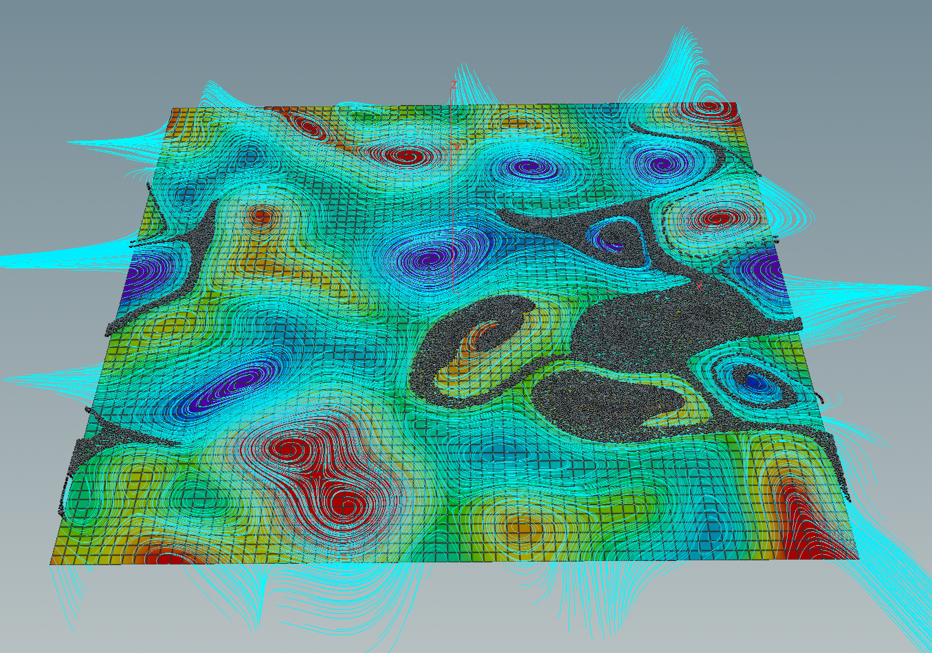
The flow of the symplectic gradient is area-preserving. A better visualization in this context would be to seed a bunch of particles uniformly in some given region. Therefore we first place a geometry in the torus – the region we want to let flow. This geometry can then be convert into uniformly distributed set of points by a scatter node. Below what this yields applied to a circle.
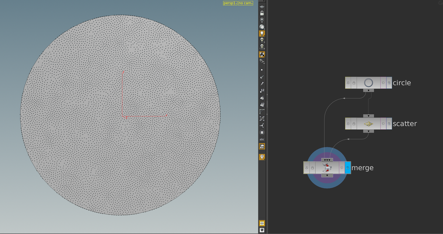
So let us put this circle in the torus and create a uniformly distributed particle cloud representing the circle.
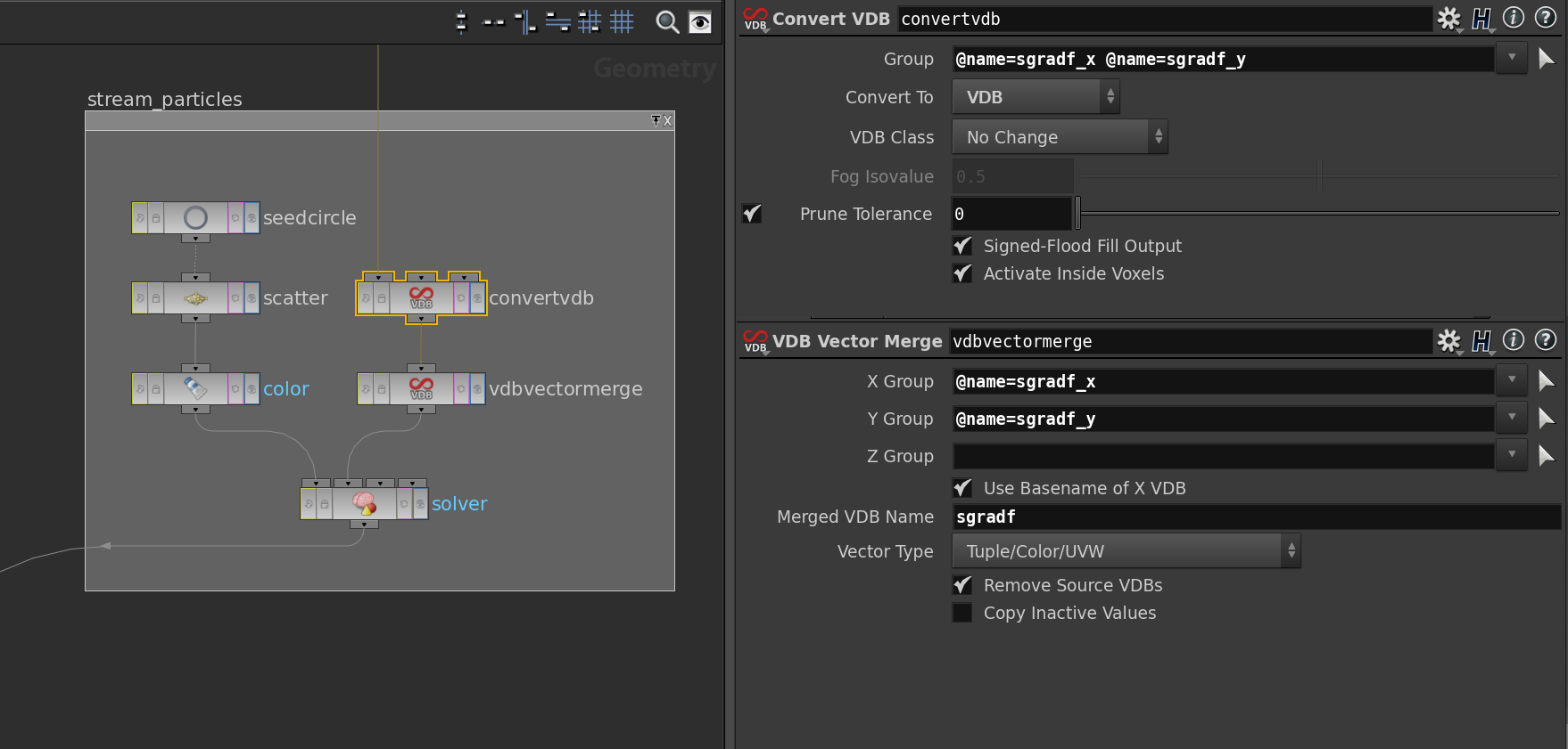
The outcome of the scatter node is then plugged into the first slot of a solver node. Further we convert the vector field into a VDB volume this we do in two steps: First we convert the components into VDB volumes using the VDB Convert node, merge this into a vector field using a VDB Vector Merge node and then stick this into the second slot of a solver node. Here the network and the parameters of VDB nodes.
Let us now look into the solver node. Here we the main part is done by a VDB Advect node. This is the place where the numerical scheme and the time-step is specified.
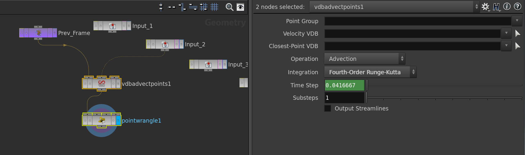
The Point wrangle node only takes care of particles leaving the torus – a bunch of if clauses which apply a suitable shift to the particles advected out of the fundamental domain.
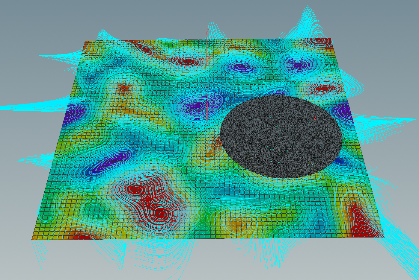
If we press then the play button down left starts to move the particles. Using a merge node we can put the torus colored by the values of \(f\) in the background.
Homework (due 21/23 June): Write a network that generates a smoothed random function and visualize the flow of its symplectic gradient using particles.