If you google “mathematics visualization”, the resulting wikipedia page shows the Mandelbrot set as a famous example.
The Mandelbrot set \(M\subset{\Bbb C}\) is defined as the following. For each \(c\in {\Bbb C}\), consider the iteration \(z_{n+1}(c) = ({z_n}(c))^2+c\), \(n=0,1,2,\ldots\) and \(z_0(c) = 0\). Observe that if \(|c|\) is small, say 0.1, then this iteration yields a sequence \(z_n(c)\) that remains bounded as \(n\rightarrow \infty\). If \(|c|\) is large, say greater than 2, then \(|z_n(c)|\rightarrow \infty\) as \(n\rightarrow \infty\). The Mandelbrot set \(M\) is the set of \(c\) which results in a bounded sequence \(z_n(c)\).
Most visualizations of Mandelbrot set you could find on web are colorful images on \({\Bbb C}\). The color at \(c\) usually indicates the number of iterations it takes before \(|z_n(c)|\) exceeds 2 (which implies \(c\) must not be in \(M\)). More precisely, people plot the function \(k:{\Bbb C}\rightarrow {\Bbb N}\cup\{0\}\)
\[k(c):=
\begin{cases}
0,& c\in \overline M\\
\min\big\{n\,\big|\, |z_{n}|>2\big\},& c\neq \overline M.
\end{cases}
\]
The algorithm for generating such \(k\) is straightforward.
- Put a grid of points \(\{c_j\}\subset {\Bbb C}\) (the points on which you want to evaluate \(k\)).
- Initialize \(k_j = 0\). (This \(k_j\) means \(k(c_j)\)). Initialize \(z_j = 0\). Initialize iteration number \(n=0\).
- Now repeat the following
- Replace \(n\) by \(n+1\);
- For each point \(j\), if \(k_j=0\), then
- replace \(z_j\) by \(z_j^2+c_j\),
- if \(|z_j|>2\) then set \(k_j=n\).
Implementing Mandelbrot set in Houdini would be a good exercise for
- creating point attributes representing complex numbers.
- iterations.
- writing functions which implements squaring complex numbers.
Step 1. Create a grid and assign point attributes
In /obj/ network port create a Geometry. Dive in this geo1, delete the default file1 node, and create a Grid. Choose its orientation “ZX Plane” with size 3\(\times\)3 centered at \((0,0,-0.5)\). Set Rows and Columns 100\(\times\) 100. After everything works, you may increase rows and columns.
Create a PointWrangle node downstream of grid1. Make sure the option “Run Over” is “Points”. Write code
|
1 2 3 4 5 6 7 |
u@z; // this creates a new attribute named z of type vector2. // we use Houdini's type vector2 to represent complex numbers @z.x=0;@z.y=0; // initialize the two component to zero. u@c; @c.x=@P.z; @c.y=@P.x; // set c to be grid point position // (note that we work on ZX plane) i@k=0; // integer attribute k. |
Here we created 3 point attributes: @z, @c and @k. Variables with prefix @ indicates that it is really some data defined on, in this case, each point. These variables would be pass to next node downstream; on the contrary variables without the prefix @ are local variables. For instance @P is the point position (of type “vector”) that has been defined. To define new attribute named name, write f@name for float data type, i@name for int data type, v@name for vector data type… See “Accessing Geometry Attributes” in the following page
http://www.sidefx.com/docs/houdini15.0/vex/snippets#attributes
In particular, the “vector2” data type is a natural choice for complex numbers. For a variable A of type “vector2”, its component is accessed as “A.x and A.y“, or equivalently “A.u and A.v“.
If you have a 3-button mouse with middle click as an ordinary middle click, long press your middle button on this PointWrangle node to observe the newly created attributes.
Step 2. Build an iteration
There are a few ways to run iterations in Houdini. One way is to use “ForLoop” node. Another way is to turn the “time line” of Houdini into our iteration. We will use the latter approach.
Create a Solver node downstream of the above PointWrangle node. Dive into this solver node. You will observe a (purple) node labeled “Previous Frame”. As one plays animation, this “Previous Frame” node takes data of the “rendered” node of the previous time frame, which allows us to implement iteration.
One also sees that the path of this solver node is quite complicated: /obj/geo1/solver1/d/s. Recall that in /obj there are only limited nodes one could create; that is the land of objects where one creates geometry node or camera or lights. In /obj/geo1 one can create all “SOP nodes” (the nodes we would be working mostly); this is a SOP land or (the land of geometry). You could take a look at /obj/geo1/solver1, it is also a land of SOP. But in /obj/geo1/solver1/d, it is a “DOP land”, the land of dynamics. The nodes you could create in a DOP land is very different from that in SOP land. It contains drivers that are related to the Houdini time line. There is a particular DOP node called “SOP solver” which is a subnetwork in which one has again an SOP land. Before you learn how to take control of DOP network, you don’t need to know any of these details. This solver node already build the DOP part for you, and all you need is to work in /obj/geo1/solver1/d/s, which is an SOP land.
Here is an important trick. Go to /obj/geo1/solver1/d, and on the parameter board, uncheck “Solve Objects on Creation Frame”. If it is checked, then at Frame 1 it would show the result already after one iteration; we uncheck it because usually we want to look at the initial state at Frame 1.
Let us return to /obj/geo1/solver1/d/s. Create a PointWrangle node. This is where we implement the algorithm for Mandelbrot set. Recall that in the algorithm, we need the iterator \(n\). In our case \(n\) is the frame number. We would like to access Houdini’s frame number. Here is a robust way of doing so:
- On the top-right of the parameter panel of this PointWrangle node, you can see a “gear” icon; click on it and choose “Edit parameter interface…”.
- You should see a window with 3 columns. On the left (Create Parameter) find the item “Integer”. Drag the “Integer” to the middle column (Existing Parameter) and insert it right above the Code folder.
- The right column (Parameter Description) shows the property of this newly created UI. Change the “Name” to
n, and change the label to whatever you want (I’ll make itnas well). Click Apply or Accept and close the window. You should see a new slider of integer is created. When your mouse curser runs over its label, you should see “Parameter: n“. - Now, in the box for entering values of
n, type$F. This is the global variable of time frame which can be called from these value boxes.
Now we can write code in the VEX expression box.
|
1 2 3 4 5 6 7 8 9 10 11 12 13 14 15 16 17 18 19 20 21 |
// First we define some helper functions vector2 square(vector2 z){ vector2 w; w.x = z.x * z.x-z.y * z.y; w.y = 2* z.x * z.y; return w; } float abs(vector2 z){ return sqrt(z.x * z.x + z.y * z.y); } // Here is the main code int n = chi("n"); // this grabs the value from the channel named n. if(@k==0){ u@z = square(u@z)+u@c; if(abs(u@z) > 2){ @k=n; } } |
If you happen to copy this code, make sure you have the “>” symbol fixed (WordPress doesn’t let me type the ordinary “>” symbol).
Note that every time I refer to the data @z, I explicitly write it with prefix u@z to keep declaring it is a vector2 variable. Sometimes Houdini just forgets the type of attributes and treat them as floats, creating some hard-to-find bugs. (Likewise one could also replace @k with i@k).
Finally, make this PointWrangle node rendered (turn the blue light on).
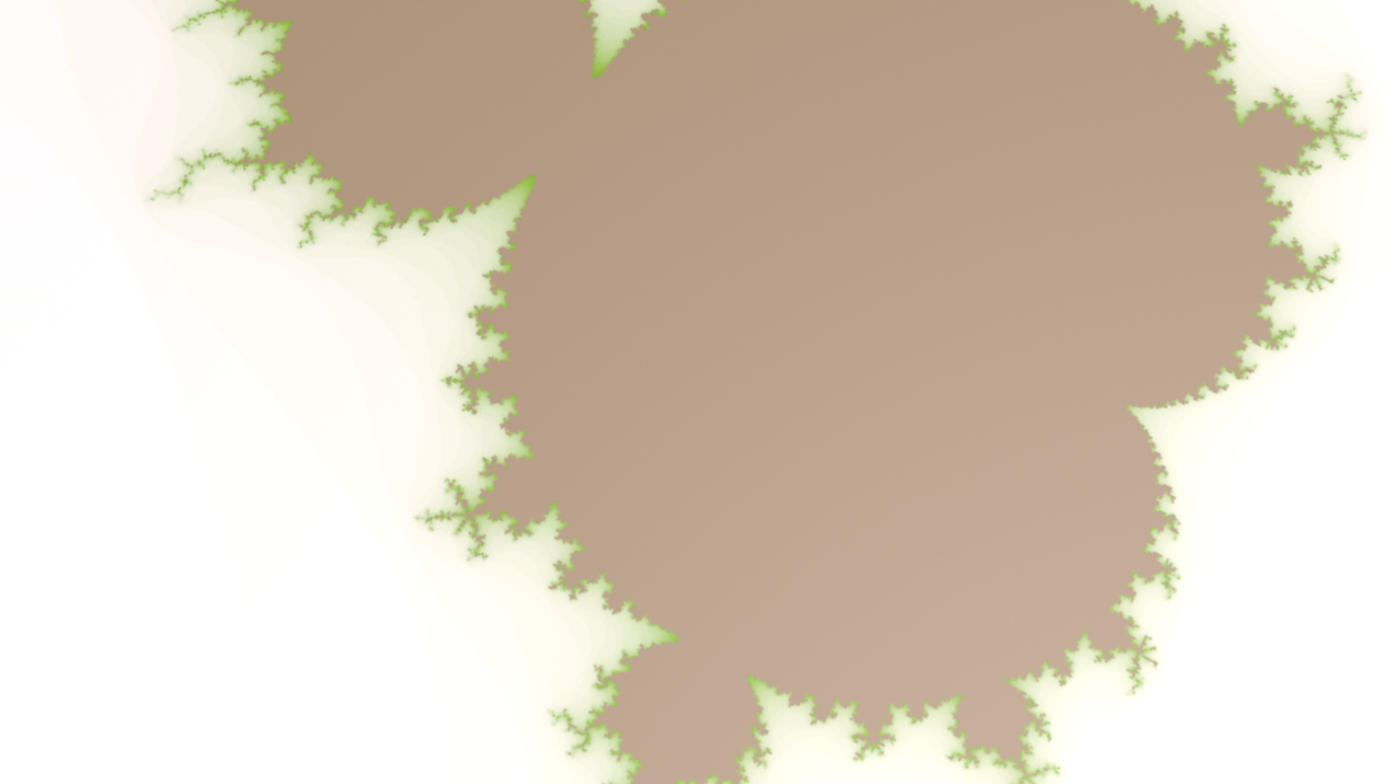
Step 3. Visualize the function k
Go back to /obj/geo1 and create another PointWrangle node downstream of the solver node. Click the gear icon \(\rightarrow\) edit parameter interface…, drag and drop a “Ramp (color)” parameter into the existing parameter column (right above the code folder). Name it “colorbar”. Accept and go back to the wrangle node. You can design your own colorbar using this UI.
In the VEX expression, type
|
1 |
@Cd = chramp('colorbar',@k/50); |
Finally, if no error has been made, play animation. One should obtain a visualization of the Mandelbrot set:
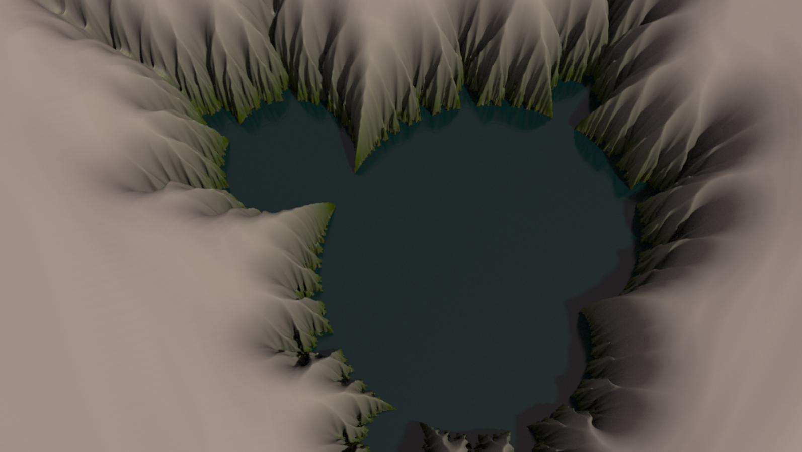
Additional fun visualization
You may find that some part of the Mandelbrot fractal looks similar to the terrain of mountains and creeks. How about really creating such terrain in Houdini?
Go back into the Solver node. Create a “Soft Transform” node. In the “Group” box, type @k=$F. In the “translate” y-channel, type -0.2/$F. In the “Soft Radius”, type 1/$F.