
It is amazingly simple to create high-quality renderings with Houdini. Several small tricks to achieve nice renderings of geometries in a mathematical context are already described in the first posts of this blog. If you not have looked at it yet you should do it now.
- Visualizing Discrete Geometry with Houdini I
- Rendering and working with Cameras
- Visualizing Discrete Geometry with Houdini II
- Simple Ambient Scenes
- Scenes with White Background
All these posts use standard geometries that come with Houdini. But how do we get other geometries into the scene?
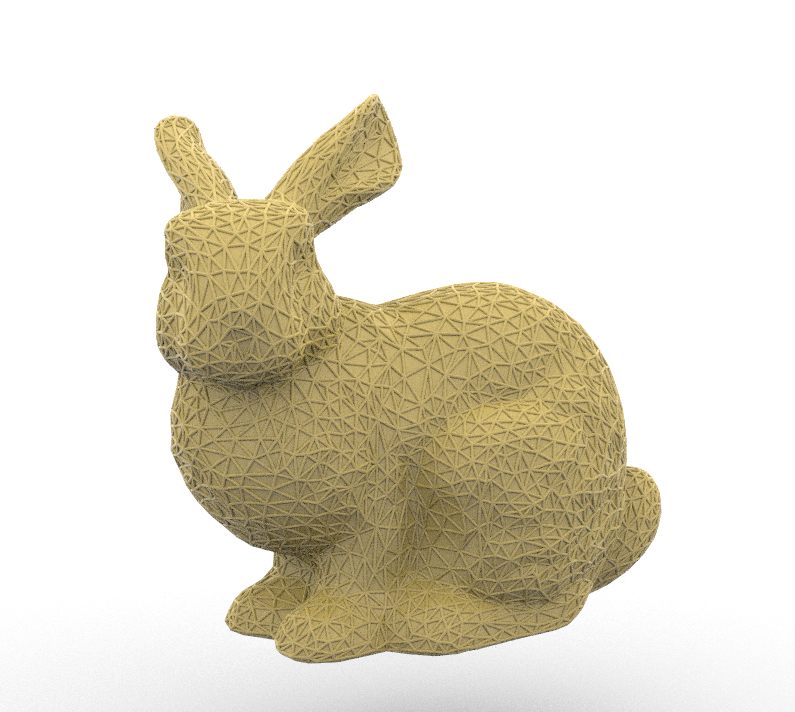
General geometries can be loaded from files (like the Stanford bunny object file). To load the file manually you can use the menu bar: Go to File \(\rightarrow\) Import\(\rightarrow\) Geometry and choose the path of your geometry file. This action creates a geometry node with a file node inside that contains the path. Instead using the menu, one can also use the file node directly. This way we can access geometry files from inside existing networks. A large library of geometry models can be found e.g. at the AIM@SHAPE website.
Now let us focus on more mathematical surfaces and how to create them using Houdini.
Small geometries can be built up easily using vex code surrounded by an Attribute Wrangle node. A detailed description how this works is given in the post Creating Geometry from Scratch.
Exercise: Play through the examples in “Creating Geometry from Scratch” and additionally build up a network that generates a cube. Choose some materials and colors to create a nice rendering.
Certainly, for larger geometries this way to construct geometries can get arbitrarily complicated and tedious.
A natural source of surfaces in space is the constant rank theorem. For maps between Euclidean space it tells us that if \(f\colon U \to \mathbb R^m\), defined on an open \(U\subset\mathbb R^n\), is a smooth map of constant rank \(k\), then \[\mathrm M = f^{-1}(\{q\}),\quad q\in \mathbb R^m\] is an \((n-k)\)-dimensional submanifold. In particular if \(f\colon \mathbb R^3 \supset U \to \mathbb R\) has full rank, then \(\mathrm M\) is a surface in \(\mathbb R^3\).
Actually Houdini offers a simple node that allows to create such implicit surfaces. It is called IsoSurface. Here one can specify a function in the coordinates \(\$X\), \(\$Y\) and \(\$Z\) on a volume (3D grid) of a certain size and resolution. Houdini then automatically generates the discrete surface that corresponds to the zero set of the given function.
Since the values in the volume are interpolated from the values at the points, the resolution of the grid has strong influence on the quality of the result. If necessary the extracted discrete surface can be post-processed with a Remesh node to obtain a triangulation.
Exercise: Create a small network that uses the IsoSurface node to generate a triangulation of a round cylinder and a torus of revolution.
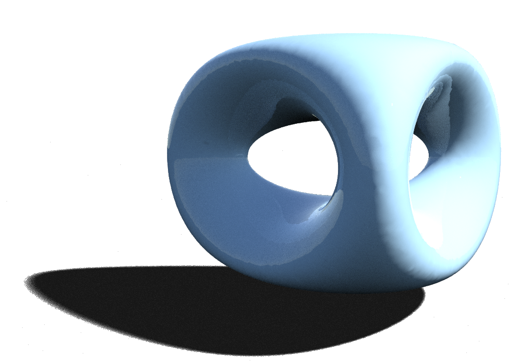
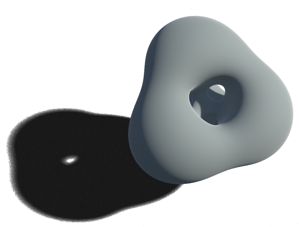
Actually there are implicit formulas to generate surfaces of arbitrary genus. For example, for the so called double-torus, a surface of genus \(2\), a formula can be found on the Wikipedia page on implicit surfaces.
In principle the surfaces and the corresponding functions could become much more complicated. Perhaps one is dealing with a discrete function which is just obtained as a numerical solution of some given problem. In this case an implicit surface can be extracted by the Convert Volume node.
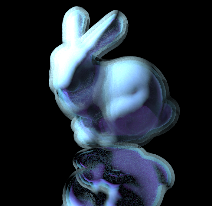
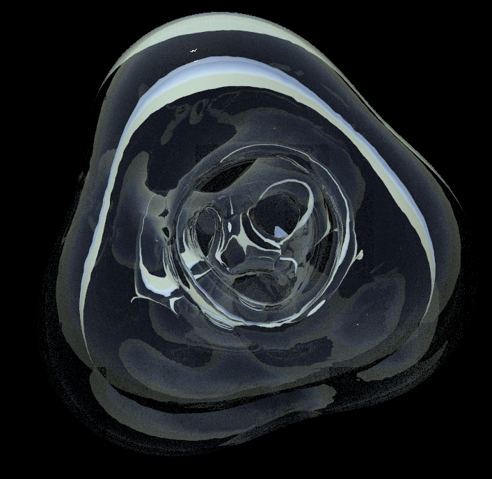
To give some illustration, the function could be e.g. the signed distance function (below the one of the Stanford bunny). From this function we extract the surface itself together with several parallel surfaces: Below a picture of the parallel surfaces – all displayed together using transparency.
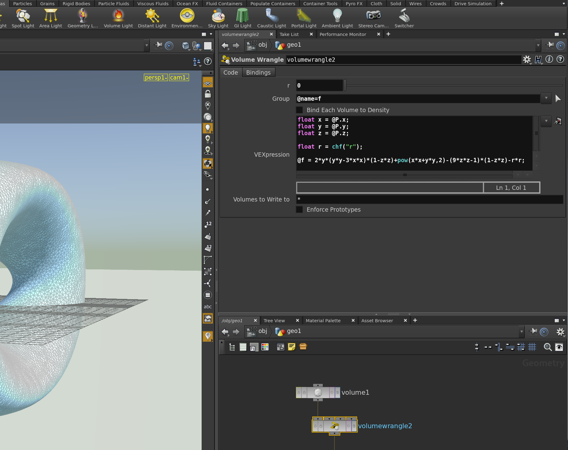
Further, given a Volume (with a specified name), we can use a Volume Wrangle node to write the function values to its points (to set arbitrary boundary values make sure that the border type in the volume properties is set to Streak). In the picture below the volume was named f. One can see how the function values that implicitly define the double torus are written to f using the VEXExpression field of the Volume Wrangle node.
The surface also can be slightly modified by a parameter r, which we added to the node. To do this we can edit the the parameter interface of the node: Right-click on the gear right to the node’s name, choose “Edit parameter interface…”. Then the following panel appears.
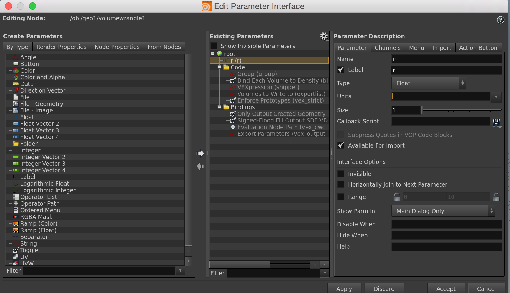
New parameters are created by drag-and-drop: Just pull the Type you need over to the field of existing parameters and give it the name/label/range you want.
Since we can now define our own functions and parameters, this gives us a huge flexibility.
Exercise: Replace the IsoSurface node in the last exercise by a system of 3 nodes – a Volume followed by a Volume Wrangle and a Convert Volume node. Add a float parameter to the parameter interface of the Volume Wrangle which allows to change the radii of the torus.
The Clebsch surface is an algebraic surface in the \(3\)-sphere. Consider the round \(3\)-sphere \[\mathrm S^3 \subset \mathbb R^4 \cong (1,1,1,1,1)^\perp :=\Bigl\{(x_1,…,x_5) \in \mathbb R^5\mid \sum_{i=1}^5 x_i =0\Bigr\} \subset \mathbb R^5.\]The Clebsch surface is then given by the cubic equation\[f(x_1,…,x_5) := \sum_{i=1}^5 x_i^3 =0.\]
The surface lies in the \(3\)-sphere, but we can use the stereographic projection to map it conformally into Euclidean space: If \(\sigma \colon \mathrm S^3\setminus\{\infty\} \to \mathbb R^3\) denotes the stereographic projection, then the image of the Clebsch surface under \(\sigma\) is given by the zero set of the function\[g= f\circ \sigma^{-1}.\]
So let us determine \(\sigma^{-1}\). Usually, if the \(3\)-sphere is considered to lie in \(\mathbb R^4\), the inverse stereographic projection is given by\[\bigl(x_1,x_2,x_3\bigr)\mapsto\frac{1}{\sum_{i=1}^3 x_i^2+1}\Bigl(2x_1,2x_2,2x_3,\sum_{i=1}^3 x_i^2-1\Bigr).\]The only thing that changes here is that we have identified \(\mathbb R^4\) with a hyperplane in \(\mathbb R^5\), so we still need to map \(\mathbb R^4\) isometrically to \((1,1,1,1,1)^\perp\). This amounts to finding an orthonormal basis of \((1,1,1,1,1)^\perp\). So one could for instance the Gram-Schmidt algorithm. But here we can also guess a suitable orthogonal basis: A possible choice is e.g. the following\[\begin{pmatrix} 1 \\ -1 \\ 0 \\ 0 \\ 0 \end{pmatrix}, \begin{pmatrix} 0 \\ 0 \\ 0 \\ -1 \\ 1 \end{pmatrix}, \begin{pmatrix} 1 \\ 1 \\ 0 \\ -1 \\ -1 \end{pmatrix}, \begin{pmatrix} 1 \\ 1 \\ -4 \\ 1 \\ 1 \end{pmatrix}.\]If we normalize these vectors and arrange them into a matrix this yields an isometric immersion \(\mathbb R^4\to (1,1,1,1,1)^\perp\subset \mathbb R^5\). With this we see that \(\sigma^{-1}\) has the following form:\[\sigma^{-1}\bigl(x_1,x_2,x_3\bigr)=\frac{1}{\sum_{i=1}^3 x_i^2+1}\begin{pmatrix} \tfrac{1}{\sqrt{2}} & 0 &\tfrac{1}{2} &\tfrac{1}{2\sqrt{5}} \\ -\tfrac{1}{\sqrt{2}} & 0 &\tfrac{1}{2} &\tfrac{1}{2\sqrt{5}} \\ 0 & 0 & 0 &-\tfrac{2}{\sqrt{5}} \\ 0 & -\tfrac{1}{\sqrt{2}} & -\tfrac{1}{2} &\tfrac{1}{2\sqrt{5}} \\ 0 & \tfrac{1}{\sqrt{2}} &-\tfrac{1}{2} &\tfrac{1}{2\sqrt{5}} \end{pmatrix}\begin{pmatrix}2x_1 \\ 2x_2 \\ 2x_3 \\ \sum_{i=1}^3 x_i^2-1\end{pmatrix}.\]
Homework (due 3/5 May): Visualize the Clebsch surface, i.e. write a network that creates a triangulation of the stereographically projected Clebsch surface, choose your favorite materials and colors and render the surface.