
If you have a polygonal curve, say arc-length parameterized, you might want to visualize the curve as the following rendering
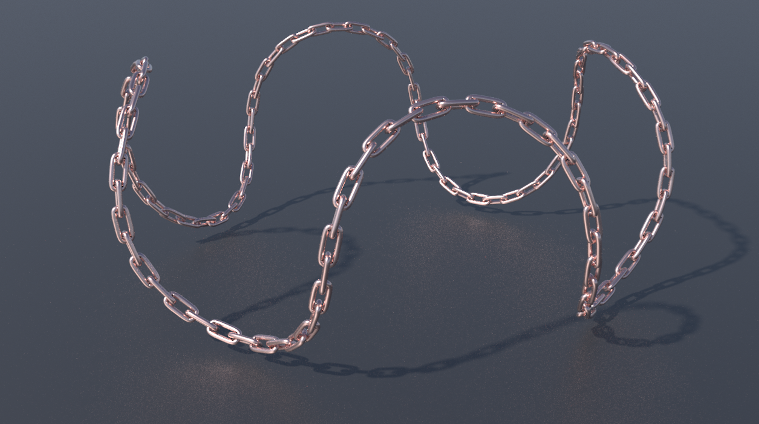
This can be done in Houdini by the “copy” SOP node.
The “copy” node has two input and one output. The first input (left input) takes a geometry that is to be copied, for instance one metal ring of the linked chain; the second input (right input) is a set of points at which the copied geometries would locate, for example the polygonal curve.
A small trick for using the “copy” node: in the copy node, go to the “Stamp” tag, and turn on “Pack geometry before copying”. It would be much more efficient and memory saving.
If you connect a piece of geometry (like the ring for the chain) to the first input of “copy” and a curve to the second input of “copy”, you would see that the rings are indeed copied and translated to the vertices of the curve. But they are not oriented as the above figure. The “copy” node creates copies of the first input and is able to transform (translate, rotate and scale) the copied geometry by reading the point attributes of the second input. For example it reads the point attribute @P (of type vector) to translate the copied geometry. To control the orientation of the copied geometry, the copy node reads the attribute @orient (of type vector4, i.e. quaternions). Since the attribute @orient has not been setup on points, it only has default orientation.
A complete list of point attributes the copy node would read can be found here
http://www.sidefx.com/docs/houdini15.0/copy/instanceattrs
Quaternions
Quaternions can represent 3D orientation (3D rotation). Quaternion \({\Bbb H}\) is a number system like complex number but with 3 imaginary dimensions; together with the real part, a quaternion is a 4-vector:
\[q\in{\Bbb H},\quad q = w+x{\bf i}+y{\bf j}+z{\bf k}\]
with multiplication rules:
\[{\bf i}^2 = {\bf j}^2 = {\bf k}^2 = -1,\quad {\bf ij}=-{\bf ji}={\bf k}, {\bf jk}=-{\bf kj}={\bf i}, {\bf ki}=-{\bf ik}={\bf j}.\]
For each 3D vector \({\bf v} = (v_x,v_y,v_z)\) one can view it as a purly imaginary quaternion \({\bf v} = v_x{\bf i}+v_y{\bf j}+v_z{\bf k}\). Then
\[q{\bf v}q^{-1}\]
is again a purely imaginary quaternion, and as a 3D vector, it is a rotation of \({\bf v}\). (Here \(q^{-1} = \overline q/|q|^2\), just like complex numbers). Quaternionic rotations are very useful because they describe rotations by “angles” and “axis to rotate about”. If you want to rotate \(\theta\) angle about an axis \({\bf a}\) (a 3D vector with \(|{\bf a}|=1\)), then the corresponding quaternion is given by
\[q = \cos\left({\theta\over 2}\right) + \sin\left({\theta\over 2}\right){\bf a}.\]
In addition, if you would like to rotate something by \(q_1\) and then by \(q_2\), the resulting rotation is simply \(q_2q_1\). This is because quaternion multiplications are associative
\[(q_2q_1){\bf v}(q_2q_1)^{-1} = q_2(q_1{\bf v}q_1^{-1})q_2^{-1}.\]
Note that quaternion multiplications are not commutative, i.e. \(q_1q_2\neq q_2q_1\) in general.
In Houdini’s VEX language, quaternions are of vector4 type. To access the components of a vector4 variable, use w (real part) and x,y,z (imaginary) fields. For example
|
1 2 3 4 5 6 7 |
vector axis = normalize({1,1,-1}); float angle = 3.14/6; vector4 Q; Q.w = cos(angle/2); Q.x = sin(angle/2) * axis.x; Q.y = sin(angle/2) * axis.y; Q.z = sin(angle/2) * axis.z; |
Fortunately, you can simplify the above code using Houdini’s VEX function vector4 quaternion(float angle, vector axis):
|
1 2 3 |
vector axis = normalize({1,1,-1}); float angle = 3.14/6; vector4 Q = quaternion(angle,axis); |
In Houdini, if you want to multiply two quaternions q1, q2, use
vector4 Q = qmultiply(q1,q2);
Parallel Frame
Now we know how to represent orientation in Houdini. We could define p@orient (p@ declares a vector4; equivalently, you may define it by vector4 @orient;) in a PointWrangle node for the curve before it enters the copy node.
But how should we orient these points on curve so that it looks most natural? Look carefully at the above rendering. Imagine each prolonged ring is a tangent vector of the curve, then two adjacent tangents form a plane (called osculating plane). Notice that two adjacent rings are just differ by a rotated within this osculating plane (rotation about the normal of osculating plane) (ignoring the \(\pi\over 2\) rotation about the tangent vector which is just for rings to interlocked). Such orientation field on a curve is called a parallel frame, i.e., there is no twist of the frame along the curve. (Chain of interlocked rings does not admit twists.)
Suppose there are \(n\) points in this polygonal curve with position \(P_0,\ldots,P_{n-1}\in{\tt vector}\). We can assign a tangent vector to each point \(T_j = {\tt normalize}(P_{j+1}-P_j)\). We would like to assign the point attribute @orient as \(Q_0,\ldots,Q_{n-1}\in{\tt vector4}\) recursively with
\[Q_{j+1} = q_jQ_j\]
where
\[q_j = {\tt quaternion}(\theta_j,{\tt axis}_j)\]
\[\theta_j = \arccos(T_j\cdot T_{j+1}),\quad{\tt axis}_j = {\tt normalize}(T_j\times T_{j+1}).\]
For the initial \(Q_0\) one could just pick any orientation; a natural choice would be
\[Q_0 = {\tt quaternion}\Big(\arccos(\{1,0,0\}\cdot T_0),{\tt normalize}(\{1,0,0\}\times T_0)\Big),\]
so that it makes sure the \(x\)-axis is always rotated to the tangent vector when using the copy node.
Sample code
After the nodes creating the curve geometry, create a PointWrangle node which we name it “compute_tangent”, and then a AttributeWrangle node which we name it “compute_parallel_frame”. In the “compute_tangent” node, make sure it “runs over points”. In the “compute_parallel_frame” node, make sure it “run over details (only once)”.
Compute_tangent:
|
1 2 3 4 5 6 7 8 |
int he = pointhedge(0,@ptnum); vector nextP = attrib(0,'point','P',hedge_dstpoint(0,he)); vector edgeVector = nextP-@P; if (he==-1){edgeVector={0,0,0};} // in case this is an end point f@pscale = length(edgeVector); v@tangent = normalize(edgeVector); p@orient; |
Compute_parallel_frame:
|
1 2 3 4 5 6 7 8 9 10 11 12 13 14 15 16 17 18 19 20 21 22 23 24 25 26 27 28 29 30 31 32 33 |
// include math.h is only for using PI #include "math.h" int n = npoints(0); // first point orientation vector xaxis = {1,0,0}; vector tangent = attrib(0,"point","tangent",0); vector rotaxis = normalize(cross(xaxis,tangent)); float rotangle = acos(dot(xaxis,tangent)); vector4 Q = quaternion(rotangle,rotaxis); setpointattrib(geoself(),"orient",0,Q); // parallel transport int currPoint = 0; vector4 cumQ=Q; do{ int he = pointhedge(0,currPoint); int nextPoint = hedge_dstpoint(0,he); if (nextPoint==-1){break;}// in case this is the end point vector currTan = attrib(0,"point","tangent",currPoint); vector nextTan = attrib(0,"point","tangent",nextPoint); rotaxis = normalize(cross(currTan,nextTan)); rotangle = acos(dot(currTan,nextTan)); Q = quaternion(rotangle,rotaxis); cumQ = qmultiply(Q,cumQ); // optional: additional twist by PI/2 for interlocking rings vector4 R = quaternion(PI/2,nextTan); cumQ = qmultiply(R,cumQ); setpointattrib(geoself(),"orient",nextPoint,cumQ); currPoint = nextPoint; }while(currPoint!=0); |
You may find that I used many functions related to “hedge” (half-edge). Look them up in Houdini’s VEX function reference. It is very useful as an iterator in polygons.