What is a typical function? The answer of this question certainly depends on the branch of mathematics you are into – while functions in differential geometry are usually smooth, the wiggling graphs appearing at the stock market are far from being so.
But how to come up with a typical smooth function? The goal of this post is to generate smoothed random functions.
A function \(f\colon \mathbb R \to \mathbb C\) is called periodic if \(f(x+2\pi) = f(x)\) for all \(x\in\mathbb R\). We define a subspace \(V\) as follows:\[\mathcal F_\infty:=\bigl\{ f\colon \mathbb R \to \mathbb C\textit{ periodic}\mid f(a_-)=\lim_{x\uparrow a}f(x),\, f(a_+)=\lim_{x\downarrow a}f(x),\, f(a) = \tfrac{f(a_+)+f(a_-)}{2}\bigr\}.\]In particular, we the demand that the one-sided limits \(\lim_{x\uparrow a}f(x))\) and \(\lim_{x\downarrow a}f(x))\) exist. On \(\mathcal F_\infty\) we have a bilinear form defined by\[\langle\!\langle f, g\rangle\!\rangle := \int_{-\pi}^{\pi}\overline{f}g .\]One can check that this form defines a hermitian inner product. Most of the properties of an inner product are obvious. Only property needs a little more care – the only if part of the positive definiteness: Suppose that \(f(a)\neq 0\), then we find \(\varepsilon, c>0\) such that \(|f(x)|^2\geq c\) for all \(x\in (a-\varepsilon,a+\varepsilon)\). Thus \(\Vert f \Vert^2 \geq \int_{a-\varepsilon}^{a+\varepsilon} |f|^2 \geq 2c\varepsilon 0\). Hence \(\langle\!\langle.,.\rangle\!\rangle\) turns \(V\) into a hermitian vector space.
We are interested in a finite-dimensional subspace \(U\subset \mathcal F_\infty\). Let us assign to each \(k\in\mathbb Z\) the function\[\mathbf e_k(x) : = \tfrac{1}{\sqrt{2\pi}}e^{i k x}.\]One easily checks that \(\mathcal S := \{\mathbf e_k\}_{k\in \mathbb Z}\subset \mathcal F_\infty\) defines an orthonormal system. The following standard theorem states that this orthonormal system is complete.
Theorem 1 (Approximation in quadratic mean). For each \(f\in \mathcal F_\infty\) and each \(\varepsilon>0\) there is \(n \in \mathbb N\) and \(c_{-n},…,c_0,…,c_n \in \mathbb C\) such that\[ \bigl\Vert f – \sum_{k=-n}^n c_k \mathbf e_k\bigr\Vert <\varepsilon.\]In other words, \(\mathcal S\) is dense in \(\mathcal F_\infty\).
This hints at that truncations of this system could be a good approximation to \(\mathcal F_\infty\): For each \(N\in\mathbb N\),\[\mathcal F_N : =\mathrm{span}_{\mathbb C}\,\{\mathbf e_k \mid |k|\leq N\}\]is a \((2N+1)\)-dimensional subspace with orthonormal basis \(\{\mathbf e_k\mid |k|<N\}\). The elements of these spaces are called Fourier polynomials.
A discrete complex-valued function on the discrete circle \(\mathfrak S^1_{2N+1}:=\mathbb Z/(2N+1)\mathbb Z\) is basically a periodic sequence \(\{a_k\}_{k\in\mathbb Z}\) with period \(2N+1\), which we can just consider as a vector in \(\mathbb C^{2N+1}\). Hence the space of discrete functions \(\mathbb C^{\mathfrak S^1_{2N+1}}\) is complex vector space of dimension \(2N+1\) as well. Again we have a hermitian inner product on this space: If \(a,b\) are discrete functions on \(\mathfrak S^1_{2N+1}\), then\[\langle\!\langle a, b\rangle\!\rangle =\tfrac{2\pi}{2N+1}\sum_{k=-N}^N \overline{a_k}b_k.\]Further we can regard the discrete circle as sitting in \(\mathbb R/2\pi\mathbb Z\). Therefore we use the map\[\iota\colon \mathfrak S^1_{2N+1}\to \mathbb R/2\pi\mathbb Z,\quad [k] \mapsto [\tfrac{2\pi}{2N+1}k].\]Certainly \(\iota\) is an injection. This allows us to define a natural linear map that assigns to each Fourier polynomial a discrete function as follows:\[V_N\ni f \mapsto f\circ\iota \in \mathbb C^{\mathfrak S^1_{2N+1}}.\]This is basically just sampling the function: If \(f\in \mathcal F_N\), then the corresponding discrete function is the sequence \(\{f(\tfrac{2\pi k}{2N+1})\}_{k\in\mathbb Z}\). Actually one can check that this map is unitary, i.e. it is an isomorphism which preserves the hermitian product. To see this let us compute it with respect to orthonormal bases: Let \(q:= e^\frac{2\pi i}{2N+1}\) and let \(f = \sum_{k=-N}^N c_k \mathbf e_k\). Then, for \(k\in\{-N,…,0,…,N\}\), \[f(\iota(k)) = f(\tfrac{2\pi k}{2N+1}) = \tfrac{1}{\sqrt{2\pi}}\sum_{l=-N}^N c_l e^{\frac{2\pi i\,k l}{2N+1}} = \tfrac{1}{\sqrt{2\pi}}\sum_{l=-N}^N c_l q^{kl}.\]Note that with respect to the product above the canonical basis of \(\mathbb C^{2N+1}\) is orthogonal but the vectors have length \(\sqrt{\tfrac{2\pi}{2N+1}}\). Rescaling by \(\sqrt{\tfrac{2N+1}{2\pi}}\) then yields an orthonormal basis \(\tilde{\mathbf e}_k\) for the discrete functions. Then with the last equation we get\[\sum_{k=-N}^N a_k \tilde{\mathbf e}_k =\sum_{k=-N}^N f(\iota(k)) \sqrt{\tfrac{2\pi}{2N+1}}\tilde{\mathbf e}_k = \sum_{k=-N}^N \Bigl(\tfrac{1}{\sqrt{2N+1}}\sum_{l=-N}^N q^{kl}c_l\Bigr)\tilde{\mathbf e}_k .\]This we can write as a matrix multiplication\[\begin{pmatrix}a_{-N}\\\vdots\\a_0\\\vdots\\a_N\end{pmatrix} = \underbrace{\tfrac{1}{\sqrt{2N+1}}\begin{pmatrix}
q^{(-N)(-N)} & \cdots & q^{(-N)0}& \cdots &q^{(-N)N}\\
\vdots & & \vdots& &\vdots\\
q^{0(-N)} & \cdots & q^{00}& \cdots &q^{0N}\\
\vdots & & \vdots& &\vdots \\
q^{n(-N)} & \cdots & q^{N0}& \cdots &q^{NN}
\end{pmatrix}}_{=:A}\begin{pmatrix}c_{-N}\\\vdots\\c_0\\\vdots\\c_N\end{pmatrix}.\]
Lemma 1. For each \(0\neq k\in\mathbb Z\) we have \(\sum_{l=-N}^N q^{kl}=0\).
Proof. Let \(z:=q^k\) and \(w:=\sum_{l=-N}^N q^{kl} = \sum_{l=-N}^N z^{l}\). Then we have\[(1-z)w = z^{-N}-z^{N+1} = (1-z^{2N+1})z^{-N} = 1.\] With \(z\neq 1\) we then get \(w=0\). \(\square\)
Theorem 2. The matrix \(A= \tfrac{1}{\sqrt{2N+1}}(q^{kl})_{k,l=-N,…,0,…,N}\) is unitary.
Proof. For \(j\neq k\) we get with the previous lemma\[(A^\ast A)_{jk} = \tfrac{1}{2N+1}\sum_{l=-N}^N q^{-jl}q^{lk} = \tfrac{1}{2N+1}\sum_{l=-N}^N q^{l(k-j)} = 0.\]Clearly, \((A^\ast A)_{jj}=1\). \(\square\)
The map \(f\mapsto f\circ \iota\) is called the inverse discrete Fourier transform (iDFT) and the theorem above can be rephrased as follows.
Corollary 1. The discrete Fourier transform (DFT) is unitary.
There is a fast algorithm to compute the DFT, which is called the fast Fourier transformation (FFT). This algorithm is standard and also Houdini provides a node for FFT on volumes.
Note that the whole setup is not restrictive to complex-valued periodic functions on the real line: real-valued functions can be considered as the real-parts of functions in \(V\) and the domain can be chosen to be a torus of arbitrary dimension. E.g. on the 3-dimensional torus \(\mathrm R^3 /2\pi\mathbb Z^3\) the corresponding othonormal system of real valued functions then consists of functions of the following form: For \(k\in\mathbb Z^3\),\begin{align*}\mathbf e_{k}^{re}(x) &= \tfrac{1}{\sqrt{2\pi}^n}\cos \bigl(\sum_{j=1}^3 k_j x_j\bigr) = \tfrac{1}{\sqrt{2\pi}^n}\cos \bigl(\langle k,x\rangle\bigr),\\ \mathbf e_{k}^{im}(x) &= \tfrac{1}{\sqrt{2\pi}^n}\sin
\bigl(\sum_{j=1}^3 k_j x_j\bigr) = \tfrac{1}{\sqrt{2\pi}^n}\sin \bigl(\langle k,x\rangle\bigr).
\end{align*}Let us stick for now with real-valued functions \(\mathcal F_N^{\mathbb R} := \{\mathrm{Re}\, f \mid f \in \mathcal F_N\}\) and focus on picking random functions.
Actually, we are only interested in the shape of the function, i.e. to us functions matter only up to scale. In particular we can assume that the functions lie on the unit sphere. We consider here uniformly distributed functions, i.e. the corresponding probability measure is rotationally symmetric and thus equals up to a constant to the standard measure on the round sphere. Corollary 1 then implies that picking a uniformly distributed random function in \(\mathcal F_N\) is the same as picking a uniformly distributed random discrete function. But how can this be done?
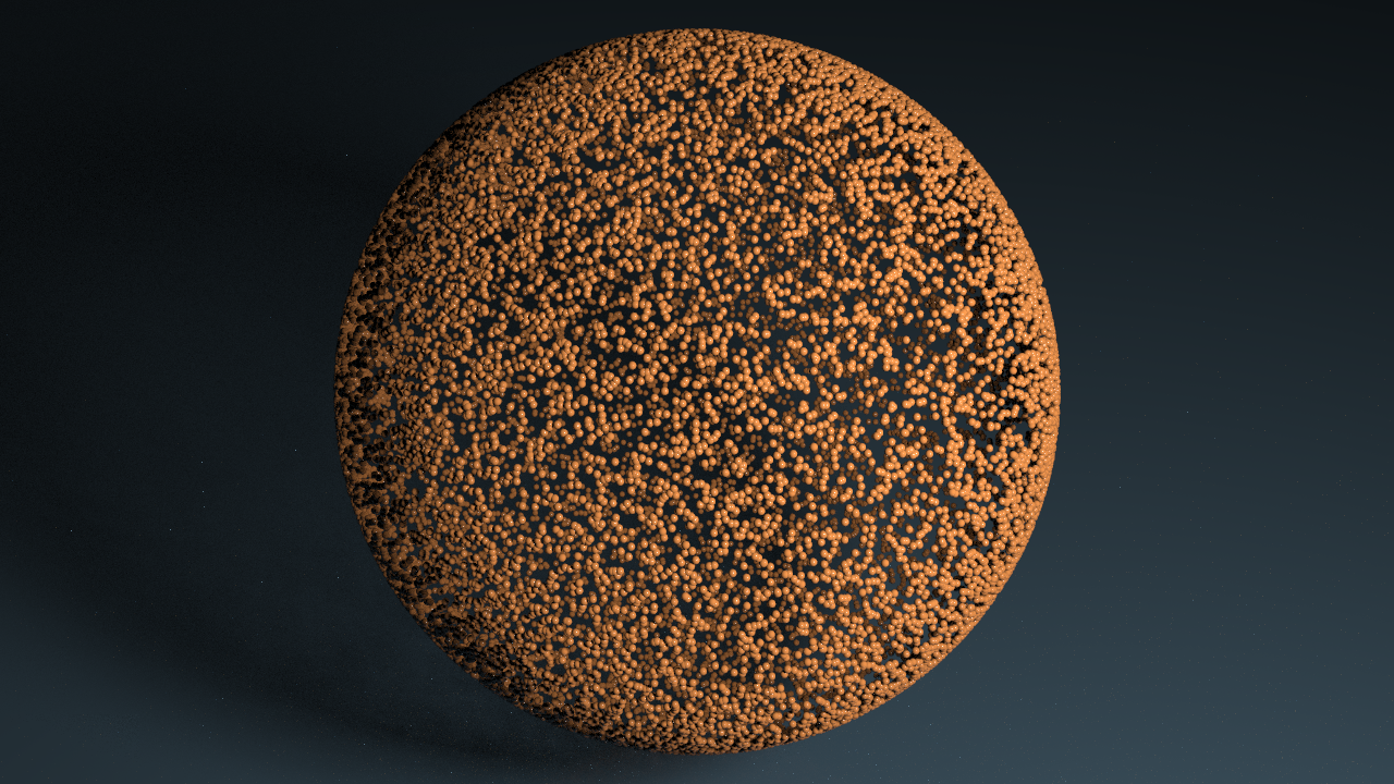
Let us first start with an example in a smaller space – the 2-sphere – and ask the same question: How to pick a random point on \(\mathrm S^2 \subset \mathbb R^3\)?
One possibility would be to choose an area-preserving map \([0,1]^2 \to \mathrm S^2\). Then picking random numbers in [0,1]^2 yields uniformly distributed points on \(\mathrm S^2\). Another easier way is the following: Pick a point \(x\in \mathbb R^3\) according to the normal distribution (also Gaussian distribution) centered at \(0\) and project.
The probability measure of the normal distribution on the real line is the probability density \(p(x) = \tfrac{1}{\sqrt{\pi}}e^{-x^2}\). The probability that a point lies in an interval \([a,b]\) is then given by the integral of the measure over \([a,b]\):\[\mathcal P([a,b])= \tfrac{1}{\sqrt{\pi}}\int_a^b e^{-x^2}.\]Actually, the probability measure is analytic and has an analytic primitive function. The error function is then defined as follows:\[\mathrm{erf}(x) = \tfrac{2}{\sqrt{\pi}}\int_0^x e^{-s^2}\,ds.\]With this definition we have\[\mathcal P([a,b]) = \tfrac{1}{2}\bigl.\mathrm{erf}\bigr|_a^b.\]Further one can check that \(\mathrm{erf}\) is monotone and maps the real line onto \((-1,1)\). Thus there is an inverse error function \(\mathrm{erf}^{-1}\colon (-1,1)\to \mathbb R\). Both functions \(\mathrm{erf}\) and its inverse are important functions and are standard in VEX.
Proposition 1. If \(x\) is uniformly distributed in \([0,1]\), then \(y=\mathrm{erf}^{-1}(2x-1)\) is normally distributed in \(\mathbb R\).
Proof. The probability that \(y\) lies in \([a,b]\) equals the probability that \(x\) lies in \([c,d]\), where \(a=\mathrm{erf}^{-1}(2c-1)\) and \(b=\mathrm{erf}^{-1}(2d-1)\), i.e. \(x \in [(\mathrm{erf}(a)+1)/2,\mathrm{erf}(b)+1)/2]\). Since \(x\) was uniformly distributed, the probability equals the length of the integral, i.e. \(\tfrac{1}{2}(\mathrm{erf}(b)-\mathrm{erf}(a))\) and \(y\) is normally distributed. \(\square\)
In higher dimensions the corresponding probabilities just multiply: The probability that a randomly chosen point lies in a cube \([a_1,b_1]\times[a_2,b_2]\times[a_3,b_3]\) is just given by\begin{multline}\mathcal P([a_1,b_1]\times[a_2,b_2]\times[a_3,b_3]) = \prod_{i=1}^3\mathcal P([a_i,b_i]) = \\ \tfrac{1}{\sqrt{\pi}^3} \prod_{i=1}^3\int_{a_i}^{b_i}e^{-x_i^2}\,dx_i = \tfrac{1}{\sqrt{\pi}^3} \int_{a_3}^{b_3}\int_{a_2}^{b_2}\int_{a_1}^{b_1}e^{-|x|^2}\,dx_1dx_2dx_3.\end{multline}Simimilarly the probability measure of the normal distribution on \(\mathbb R^n\) is given by\[p(x) = \tfrac{1}{\sqrt{\pi}^n}e^{-|x|^2}\]In particular we find that the normal distribution in is rotationally invariant.
From this we see we can get a randomly sampled sphere as follows: If we choose \(y_i\in[0,1],\) \(i=1,2,3\), uniformly distributed and define \(x_i = \mathrm{erf}^{-1}(2y_i – 1)\), then \(x=(x_1,x_2,x_3)\) is normally distributed in \(\mathbb R^3\). By the rotational symmetry the point projected to the sphere is then a uniformly distributed.
This can be carried over directly to the function case – just take for each point a uniformly distributed random number in \([0,1]\) and then apply \(\mathrm{erf}^{-1}\) as above.
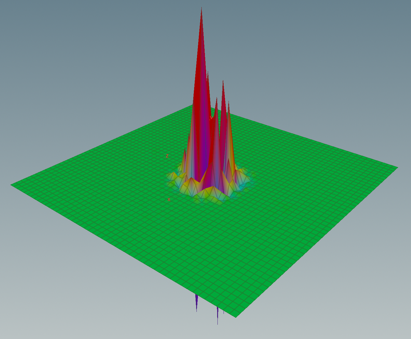
The FFT maps uniformly distributed random discrete functions to uniformly distributed functions in Fourier domain. Hence if we apply the FFT to a random function nothing changes – we have the same look and feel.
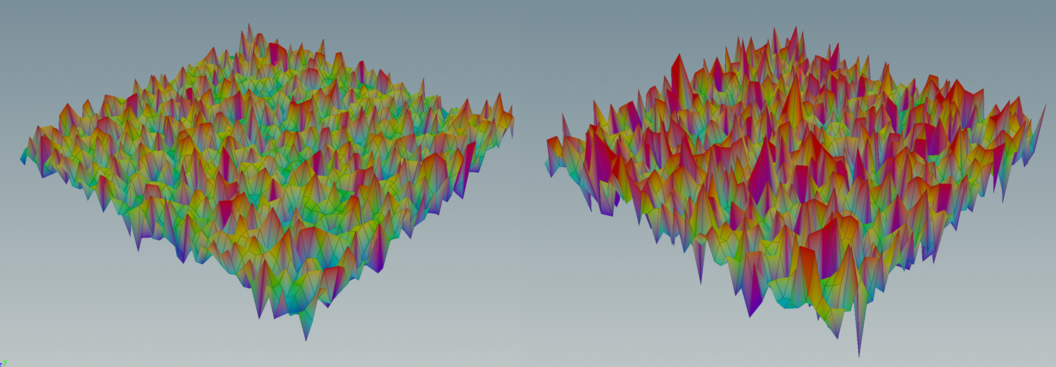
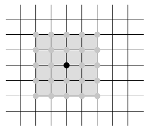
Certainly, we rather prefer some smooth functions. For now we just use a simple blur, i.e. we just average the values over a stencil like the following
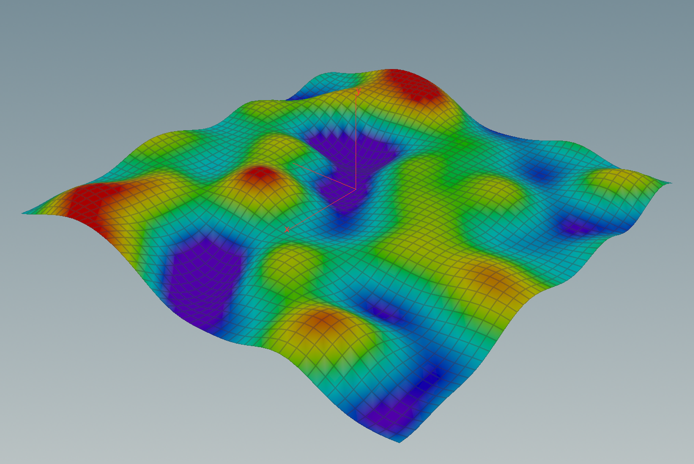
The resulting functions then look e.g. as follows:
If we now apply the FFT then the function changes drastically – now the values concentrate around the center, i.e. the coefficients are larger for low frequencies.