
A discrete curve \(\gamma\) in a space \(\mathrm M\) is just a finite sequence of points in \(\mathrm M\), \(\gamma = (\gamma_0,…,\gamma_{n-1})\). In case we have discrete curve \(\gamma\) in \(\mathbb R^3\) we can simply draw \(\gamma\) by joining the points by straight edge segments.
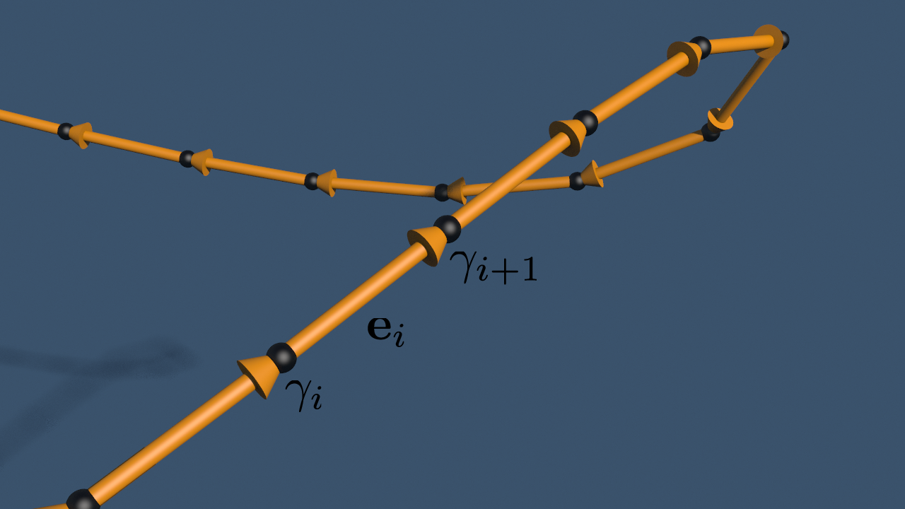
The vector that moves a point \(\gamma_i\) to the next point \(\gamma_{i+1}\) is called the discrete tangent vector \[\mathbf e_i := \gamma_{i+1}-\gamma_i.\]Further, the normalized tangent vector will be denoted by\[T_i := \frac{\mathbf e_i}{\Vert\mathbf e_i\Vert}.\]It is even more convenient to draw the points as small spheres and the lines as tubes that align with the corresponding edge. Actually there is 1-parameter freedom to place the tube around the edge – we could rotate the tube around the edge – which is hidden in the tube’s rotational symmetry.
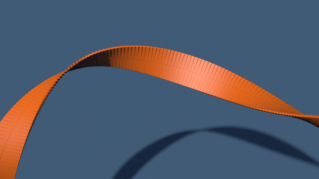
If we instead would like replace the edges by a less symmetric shape (as e.g. in Albert’s post) or if we want to really mesh a tubular surface around the curve this freedom matters. Therefore we must additionally specify a direction in the normal space of the edge.
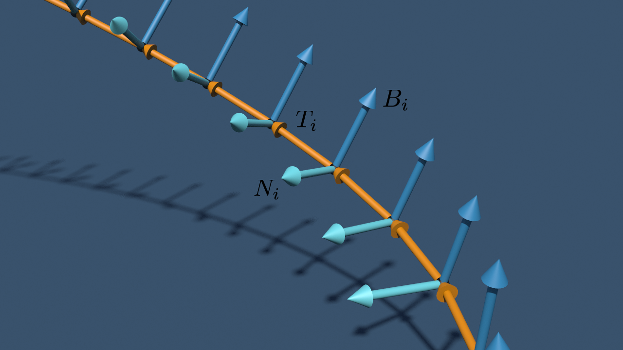
A discrete normal vector field of \(\gamma\) is a sequence \(N= (N_0,…,N_{n-2})\) such that\[N_i\perp T_i, \textit{ for all }i=0,…,n-2.\]For convenience, \(\mathcal N_i:=T_i^\perp\). Given such a discrete normal vector field \(N\) we automatically obtain a second normal vector field from it:\[B := T\times N.\]The triple \(\sigma= (T,N,B)\) then yields at each vertex an oriented orthonormal basis of \(\mathbb R^3\), where the first vector aligns with the tangent direction. This kind of object are well-known in differential geometry and in analogy to the smooth case we will call it a discrete frame.
Like in the smooth case, there are distinguished frames among all the possible ones. A quite old-fashioned but still famous notion is the Frenet frame (see e.g. this wikipedia entry). We will instead work with parallel frames here:
The discrete parallel transport is map that assigns to each point \(i\) a rotation \(P_i\in \mathrm{SO}(3)\) that describes how the normal spaces \(\mathcal N_{i-1}\) and \(\mathcal N_i\) are connected: If \(T_{i-1}\times T_i = 0\) we set \(P_i=\mathrm{id}\), else \(P_i\) is the unique rotation around \(T_{i-1}\times T_i\) that maps \(T_{i-1}\) to \(T_i\), i.e.\[P_i(T_{i-1}) = T_i, \quad P_i(T_{i-1}\times T_i) = T_{i-1}\times T_i.\]Now, let \(N\) be a discrete normal vector field of the discrete curve \(\gamma\). We say \(N\) is parallel, if \[N_i = P_i(N_{i-1}), \quad i =1,…,n-2.\]A parallel discrete frame is then a discrete frame \((T,N,B)\), where \(N\) (and consequently \(B\)) is a parallel discrete normal vector field.
In Houdini rotations are stored as quaternions. So it is convenient to describe the parallel transport in quaternions, i.e. we want to find \(q_i\in \mathbb H\), \(\Vert q_i\Vert=1\) such that \[P_i(X)= q_i\,X\,\overline{ q_i}, \quad X \in \mathcal N_{i-1}.\]Here we identified \(\mathbb R^3\) with the imaginary quaternions (compare with Albert’s post):\[\mathbb R^3 \ni (x,y,y) \longleftrightarrow x\,\mathbf i + y\,\mathbf j + z\,\mathbf k \in\mathrm{Im}(\mathbb H).\]Now let us find a formula for \(q_i\). First, recall that if \(\mathbf v\in \mathbb R^3\), \(\Vert \mathbf v\Vert=1\), then the rotation around \(\mathbf v\) by the angle \(\alpha \in\mathbb R\) is given by the quaternion\[\cos\bigl(\frac{\alpha}{2}\bigr) + \sin\bigl(\frac{\alpha}{2}\bigr)\mathbf v .\]
The first condition on \(P_i\) tell us that \(q_i = a_i + \mathbf v_i\) where \(\mathbf v_i \perp T_{i-1},T_i\). In particular, \(T_{i-1}\overline{q}_i = q_i\, T_{i-1}\). The second condition then yields that \[T_i = q_i\, T_{i-1}\, \overline{q}_i =q_i^2\, T_{i-1}\]and hence\[\bigl(a_i^2 – \Vert\mathbf v_i\Vert^2\bigr) +2a_i \mathbf v_i = q_i^2 = -T_i T_{i-1} = \langle T_i,T_{i-1}\rangle – \mathrm{Im}\bigl(T_iT_{i-1}\bigr).\]Here we used that \(T_{i-1}^{-1}= -T_{i-1}\). Further, since \(\Vert q_i\Vert =1\), we obtain \(1 – a_i^2= \Vert \mathbf v_i\Vert\), which we can substitute into the equation above. Comparing real and imaginary part then yields two equations\[a_i^2 =\frac{1+\langle T_i,T_{i-1}\rangle}{2}, \quad \mathbf v_i = -\frac{1}{2a_i}\mathrm{Im}\bigl(T_iT_{i-1}\bigr).\]
Note that the equation above determines \(q_i\) only up to sign. Therefore we can assume that \(a_i\geq 0\). Hence we end up with the following formula for \(a_i\) and \(\mathbf v_i\):\[a_i = \sqrt{\frac{1+\langle T_i,T_{i-1}\rangle}{2}},\quad \mathbf v_i = \frac{-1}{\sqrt{2+2\langle T_i,T_{i-1}\rangle}}\mathrm{Im}\bigl(T_iT_{i-1}\bigr).\]
Now given the discrete parallel transports we can easily construct a parallel normal field \(N\) as follows: Choose some vector \(N_0\) normal to the first edge. Then propagate this vector to the whole curve using the transport,\[N_i := P_i\circ\cdots\circ P_1(N_0) = \underbrace{q_i\cdots q_1}_{=:\mathfrak q_{0,i}} \,N_0\, \overline{q}_1\cdots \overline{q}_i =\mathfrak q_{0,i}\, N_0 \, \overline{\mathfrak q_{0,i}}.\]
Actually that is what is used by Albert to orient the chain links: The chain link is a fixed geometry in its own coordinate system. The copy node makes for each point a copy which is then translated to the current point’s position and stretched by the attribute @pscale. If the node finds an attribute named @orient (a quaternion store as vector4), it additionally performs the corresponding rotation. Hence if the chain was aligned with the \(x\)-axis (i.e. with the quaternion \(\mathbf i\)) we need to specify quaternions that rotate the vector \(\mathbf i\) to the corresponding tangent vectors \(T\). Therefore we can choose any quaternion, say \(\psi_0\), to get the rotation from \(\mathbf i\) to the first edge \(T_0\),\[T_0 = \psi_o\mathbf i\,\overline{\psi_o},\]before we use the parallel transports \(q_i\) to get the other rotations:\[\psi_i := q_i\cdots q_1\psi_0.\]
Homework (due 10/12 May): Rebuild the chain rendering presented in the previous post. Write two networks: one using the closed arclength-parametrized curves from Ulrich’s post, and a second one that uses the curve node to build up a generic closed curve as input. (Use the resample node to make it arclength-parametrized).