Wave- and heat-equation on surfaces

Wave equation

Let $M$ be a surface and $f : \mathbb{R} \times M \rightarrow \mathbb{R}$ a function. The wave equation is given by:
\[\ddot{f} = \Delta f.\]
After the space discretization we have $f:\mathbb{R} \times V \rightarrow \mathbb{R},$ $p:= \left(\begin{matrix} f_1 \\ \vdots \\ f_n \end{matrix} \right) \in \mathbb{R}^n$ and $\Delta \in \mathbb{R}^{n \times n}$, where $n:=|V|$ denotes the number of vertices. Therefore, the wave equation becomes a linear system of second order ODE’s. In the last lecture we saw that the Verlet method works well for second order ODE’s. Using this for the Wave equation we get:\[\frac{p_{k-1}-2 p_k + p_{k+1}}{\delta^2} = \Delta p_k,\]
where $\delta$ is the time step.
For initial data $p_0,p_1$, the hope is that the energy of the system neither grows exponentially nor that the system comes to a halt. A classical example for the $1-$dimensional wave equation is an oscillating string. This leads in analogy to music instruments to two kinds of initial data:

  1. Cembalo initial data: \[p_0 = p_1,\] here the string gets plucked, i.e. at time $t=0$ the oscillation is $p_o$ and the speed is zero.
  2. Piano initial data: \[p_0 =0,\] here the string gets struck i.e.  at time $t=0$ the oscillation is zero but the speed is not.

A different way to find solutions of the wave equations is to calculate the eigenfunctions of the laplace operator, $g:M \rightarrow \mathbb{R}$:
\[\Delta g= -\omega ^2 g.\]
Since the laplace operator is symmetric and negative definite, $\Delta$ is diagonalizable and there exist eigenvalues $\lambda_i := – \omega ^2_i$ with corresponding eigenfunctions $g_i$ such that such that:
\[0 = w_o^2 < w_1^2<  w_2^2 \ldots.\]
Note that $0$ zero is an eigenvalue, because the kernel of $\Delta$ consists of the constant functions. If we computed the eigenfunctions, solutions of the wave equation can be constructed in the following way:
\[f(t,p) := \sum_{i =1}^n \left( a_i \cos(\omega_i t) + b_i \sin(\omega_i t)\right) g_i(p) , \quad \quad \quad a_i,b_i \in \mathbb{R}.\]
The coefficients $a_i$, $b_i$ have to be chosen in a way such that the initial conditions are satisfied. Note that for different surfaces the spectrum of eigenvalues is different. A sphere “sounds” different then the bunny.  The disadvantage of this method is, that finding the eigenfunctions of the surface and computing the coefficients for the initial conditions can be very expensive, especially if the surface has many vertices.

Heat equation

For $f : \mathbb{R} \times M \rightarrow \mathbb{R}$, the heat equation is given by:
\[\dot{f} = \Delta f.\]
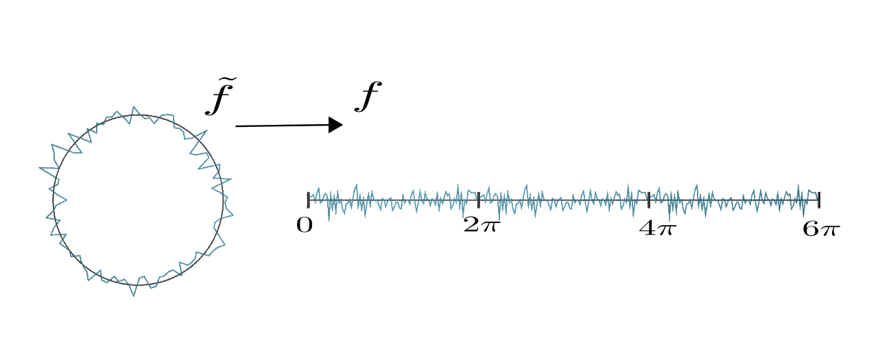
We will start our investigation by considering the case $M = \mathbb{S}^1.$ There we can describe a function $\tilde{f} : \mathbb{S}^1 \rightarrow \mathbb{R}$ by an periodic function $f : \mathbb{R} \rightarrow \mathbb{R},$ with  $f(x + 2\pi) = f(x).$

func on s1

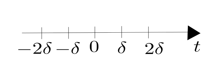
Our aim is it to use the Euler forward method to solve the heat equation on $\mathbb{S}^1$, therefore we discretize the space, i.e. the interval $[0,2\pi]$, as follows:
\[x_k = \frac{2\pi k}{n}, \quad \quad  x_{k+1} = x_k + h, \quad \quad \mbox{with }\quad h = \frac{2\pi}{n}.\]
In an earlier lecture we discussed discrete periodic functions and defined a canonical basis for them, such that we can write the components of $p_j =  \left(\begin{matrix} u_1 \\ \vdots \\u_{2n-1} \end{matrix} \right)$ as
\[u_k = \frac{1}{\sqrt{2 \pi}}\sum_{m = -n}^n a_m e^{\frac{i 2\pi km}{n}} \quad \quad a_m \in \mathbb{C}.\]
Since we are considering real valued functions there has to hold $a_m = \bar{a}_{-m}$ for all $m \in \left\{-n, \ldots,0,\ldots, n\right\}$.
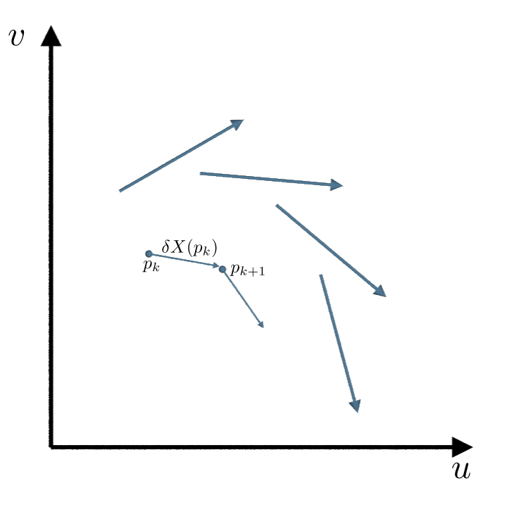
If we now use the Euler forward method we get:
\[p_{j+1} = p_j + \delta \Delta p_k,\]
where $\delta$ denotes the time step size. The discrete laplacian on $\mathbb{S}^1$ can be considered as an approximation of the second spatial derivative and is defined as:
\[\left( \Delta u\right)_k = \frac{u_{k-1} -2 u_k + u_{k+1}}{h^2}.\]
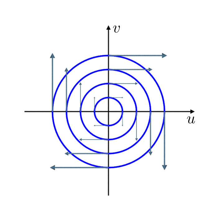
By linearity it is enough to consider the case $u_k = e^{\frac{i 2\pi km}{n}}$:

\begin{align} \tilde{u}_k & = u_k +\left( \Delta u\right)_k  \\ & = e^{\frac{i 2\pi km}{n}} + \delta \frac{ e^{\frac{i 2\pi (k-1) m}{n}}-2 e^{\frac{i 2\pi km}{n}} + e^{\frac{i 2\pi (k+1)m}{n}}}{h^2} \\ & = \left(1 + \delta \frac{e^{\frac{i 2\pi m}{n}} + e^{\frac{-i 2\pi m}{n}} + 2}{h^2} \right) e^{\frac{i 2\pi km}{n}} \\ & = \left( 1 + \frac{2\delta}{h^2}\left( \cos \left(\frac{2 \pi m}{n}\right) -1\right)\right) u_k. \end{align}
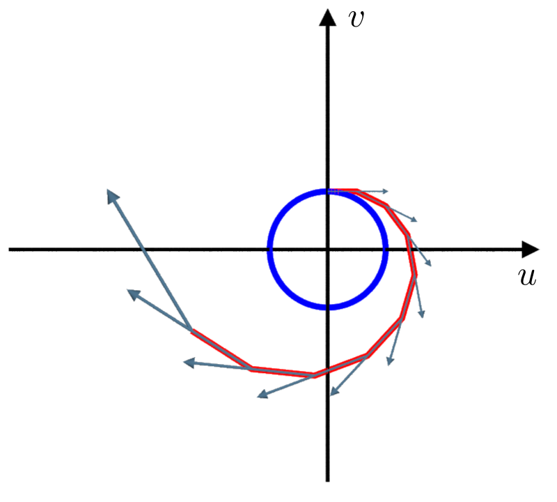
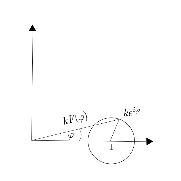
The system will blow up after a certain time if there is an $m$ such that:
\begin{align} & \left| 1 + \frac{2\delta}{h^2}\left( \cos \left(\frac{2 \pi m}{n}\right) -1\right)\right| > 1 \\ \Leftrightarrow  \quad  &\frac{2\delta}{h^2}\left( \cos \left(\frac{2 \pi m}{n}\right) -1\right) < -2.\end{align}
The left hand side reaches its minimum if $m = \frac{n}{2}$ i.e $\cos \left(\frac{2 \pi m}{n}\right) = -1$ and we get:
\begin{align} &\frac{2\delta}{h^2}> 1 \\ \Leftrightarrow \quad & \delta > \frac{h^2}{2}.\end{align}

This gives us a connection between the space and time discretization that is not wanted. If we use the Euler forward method to solve the heat equation on $\mathbb{S}^1$ and we refine the time step by the factor of $10$, we have to refine the space discretization by the factor of $50$, to avoid the solution to blow up. Therefore it makes more sense to use the Euler backward method for this problem.

Posted in Lecture | Comments Off on Wave- and heat-equation on surfaces

Partial differential equations involving time

Let $\Omega \subset \mathbb{R}^n$ be a domain, we will consider $\Omega$ to be the “space” and functions:
\begin{align}
f : \mathbb{R} \times \Omega \rightarrow \mathbb{R}, \\ (t,x) \mapsto f(t,x),\end{align}
will be view as time dependent functions
\begin{align}
& f_t : \Omega \rightarrow \mathbb{R}, \\ & f_t(x) := f(t,x).\end{align}

We want to investigate partial differential equations  (PDE’s) for $f$, that involve the Laplace operator. Here the Laplace operator is defined just for the space coordinates $x$:
\[\left(\Delta f\right) (t,x) := \left(\Delta f_t\right) (x) := \sum_{i=1}^n \frac{\partial^2 f_t(x)}{\partial x_i^2}.\]
Typical examples for such PDE’s from physics are:

  1. Wave equation: \[\frac{\partial^2 f}{\partial t^2} = c^2 \Delta f, \quad \quad \quad c \in \mathbb{R}.\]
  2. Heat equations: \[\frac{\partial f}{\partial t} = c \Delta f, \quad \quad \quad c \in \mathbb{R}.\]

We will investigate these PDS’s on closed triangulated surfaces  $\Omega = M = (V,E,F)$, where we only have finitely many function values i.e. :
\begin{align} &  f : \mathbb{R} \rightarrow \mathbb{R}^V, \\&  f(t) = \left( \begin{matrix}  f_1(t) \\ \vdots \\ f_N(t) \end{matrix} \right) .\end{align}
On $M$ we have the usual Laplace operator $\Delta :\mathbb{R}^V \rightarrow \mathbb{R}^V$ and for the above PDE’s we obtain ordinary differential equations (ODE’s):

  1. Wave equation: \[\ddot{f}(t)= c^2 \Delta f(t).\]
  2.  Heat equations: \[\dot{f}(t)= c \Delta f(t).\]

This is a big improvement since it is fare more complicated to solve PDE’s then ODE’s.
Before we will present some methods to solve ODE’S numerically consider the Pendulum equation as example:
\[\ddot{\varphi} = -\sin(\varphi).\]

pendulum

The standard procedure to solve a second order ODE is to transfer it in a system of two ODE’s of first order. Therefore consider:
\begin{align} &  f : \mathbb{R} \rightarrow \mathbb{R}^2, \\&  f(t) = \left( \begin{matrix}  \varphi (t) \\ \dot{\varphi} (t) \end{matrix} \right) .\end{align}
Then $\varphi$ solves the pendulum equation if and only if $f$ solves
\[\left( \begin{matrix}  u \\ v \end{matrix} \right)^{\bullet} = \left( \begin{matrix}  v \\ -\sin (u) \end{matrix} \right). \]
The energy of the above system is given by $E(t) := \frac{1}{2}\dot{\varphi}^2 – \cos(\varphi).$ $E$ is a constant of motion since:
\[\dot{E} = \dot{\varphi} \ddot{\varphi} + \dot{\varphi} \sin (\varphi) = o,\]

The level-sets of the energy of the pendulum. The yellow dots correspond to $E=-1$, the green curves to $-1<E<1$, the blue ones to $E=1$ and the red ones to $E>1$.

if $\varphi$ is a solution of the pendulum equation. In the phase space the solutions of the ODE are implicitly given by the level-sets of $E$ :

By the theorem of Picard-Lindelöf there is for every $\left( \begin{matrix} u_0 \\v_0 \end{matrix} \right) \in \mathbb{R}^2 $ a  unique solution of the initial value problem (IVP) :
\begin{align}  & \left( \begin{matrix}  u \\ v \end{matrix} \right)^{\bullet} = X(u,v)  = \left( \begin{matrix}  v \\ -\sin (u) \end{matrix} \right) \\ & \left( \begin{matrix}  u \\ v \end{matrix}\right)(0) = \left( \begin{matrix}  u_0 \\ v_0 \end{matrix} \right).\end{align}
These solutions lie on the level-sets of $E$.
Now we want to approximate the solution of the IVP by a sequence
\[\ldots,\left( \begin{matrix}  u_{-1} \\ v_{-1} \end{matrix} \right), \left( \begin{matrix}  u_0 \\ v_0 \end{matrix}\right) , \left( \begin{matrix}  u_1 \\ v_1 \end{matrix}  \right),\ldots \in \mathbb{R}^2\]
such that for the real solution $\left( \begin{matrix}  u(t) \\ v(t) \end{matrix}  \right)$ we have $\underbrace{\left( \begin{matrix}  u_k \\ v_k \end{matrix}  \right)}_{p_k} \approx \left( \begin{matrix}  u \\ v\end{matrix}  \right) (k\delta), $
where $\delta$ is the time step.
timedisc

There are several methods to get such a sequence:

1. Forward Euler method:

Let $ X: \mathbb{R}^2 \rightarrow \mathbb{R}^2$ be the vectorfiled representing the ODE , i.e. \[\left( \begin{matrix}  u \\ v \end{matrix} \right)^{\bullet} (k\delta)= X(u(k\delta),v(k\delta)) = X(p_k).\]

euler

Then with the forward Euler method we get from $p_k$ to $p_{k+1}$ by walking for the time $\delta$ in the direction of $ X(p_k)$.

\[p_{k+1} = p_k + \delta X(p_k).\]

The big advantage of this method is, that it is very fast. The disadvantage is illustrated in the following example: For the harmonic oscillator the ODE is given by the vectorfield:
\[X(u,v) = \left( \begin{matrix} v \\ -u \end{matrix}\right).\]
Its analytic solution is:
\[ \left( \begin{matrix} u \\ v \end{matrix}\right)(t) = \left( \begin{matrix} \cos(t) & \sin(t)\\ -\sin(t) & \cos(t)\end{matrix}\right) \left( \begin{matrix} u_o \\ v_0\end{matrix}\right)\]

The vector field and the corresponding integralcurves of the harmonic oscillator.

The energy is a again a constant of motion: $E(t) := \frac{1}{2} \left( u^2 + v^2 \right)$ and the level-sets of $E$ are circles. If we apply the forward Euler method the solution is a spiral and not a circle. Therefore, the energy gets bigger and bigger and the solution blows up.

The rela integralcurve (blue) and the one obtain with the eulerforward method for $\delta = 0.5 (red)$, together with the corresponding vectorfield (grey).

The real integralcurve (blue) and the one obtain with the Euler forward method for $\delta = 0.5$  (red), together with the corresponding vectorfield (grey).

2. Backward Euler method:

The backward Euler method works in the following way: Find $p_{k+1}$ such that one Euler forward step with respect to the vectorfield $-X$ gives you $p_k$. i.e
\[p_k = p_{k+1} -\delta X(p_{k+1}).\]
That means we have to solve the following non linear system of equations to get from $p_k$ to $p_{k+1}$:
\[p_{k+1} =  p_k + \delta X(p_{k+1}).\]

This can for example be done with the classical Newton method. The advantage of the backward Euler method is that the energy does not increase and therefore the solution does not blow up. The disadvantage is that solving a non linear system of equations can be hard and expensive.

The idea behind both Euler methods, that guaranties the convergence to the real solution for $\delta \rightarrow 0$ is given by the mean value theorem: For $f \in C^1(\mathbb{R},\mathbb{R}^n)$, $p \in \mathbb{R}$ and $\delta >0$ there exist $\tau \in (p,p+\delta)$ such that”
\[f'(\tau) = \frac{f(p)-f(p+\delta)}{\delta}.\]

3. Verlet method:

The Verlet method works for equations of the form \[\ddot{f}(t) = F\left( f(t)\right), \quad \quad \quad \quad \quad f \in C^2(\mathbb{R},\mathbb{R}^n).\]

In order to approximate $f(k\delta)$ by $p_k$ we use the mean value theorem twice:

\begin{align}\ddot{f}(t) & \approx \frac{\dot{f}\left(t+\frac{\delta}{2}\right) -\dot{f}\left(t-\frac{\delta}{2}\right)}{\delta} \approx \frac{\frac{f \left( t+\delta\right) -f \left(t\right) }{\delta} -\frac{ f \left( t\right) -f \left( t-\delta\right) }{\delta}}{\delta}\\ & = \frac{f( t + \delta) -2f(t) + f(t-\delta)}{\delta^2}.\end{align}

This gives us the following recursion formula for the $p_k$’s:
\begin{align}  F(p_k) & = \frac{p_{k-1} -2p_k + p_{k+1}}{\delta^2}\\ \Leftrightarrow  \quad p_{k+1} & = 2p_k -p_{k-1} + \delta^2 F(p_k).\end{align}

To solve this recursion formula, we start with the initial data \[ \left( \begin{matrix} p_0  \\  p_1 \end{matrix} \right) :=  \left( \begin{matrix} u_0  \\  v_1 \end{matrix}  \right) := \left( \begin{matrix} f(0)  \\  f(\delta) \end{matrix} \right) \]
with the approximation:
\begin{align} \frac{p_0 + p_1}{2} \approx f\left( \frac{\delta}{2}\right), \\ \frac{p_1-p_0}{\delta} \approx \dot{f}\left( \frac{\delta}{2}\right), \end{align}

this corresponds to the usual initial data of an IVP for a  for a second order ODE. Afterwords we use:

\[\left( \begin{matrix} p_k  \\  p_{k+1} \end{matrix}  \right) = \left( \begin{matrix} u_k  \\  v_k \end{matrix}  \right) = \left( \begin{matrix} v_{k-1}  \\  2v_{k-1} -u_{k-1} + \delta^2 F(v_{k-1}) \end{matrix}  \right) . \]

If we consider that as a two dimensional system with $q_k := \left( \begin{matrix} u_k  \\  v_k \end{matrix}  \right)$, we have:
\[q_{k+1} = X(q_k) ,\]
with:
\begin{align} & X:\mathbb{R}^2 \rightarrow \mathbb{R}^2, \\ & X(u,v)  = \left( \begin{matrix} v  \\ 2v -u + \delta^2 F(u)  \end{matrix}  \right). \end{align}

This is a very good choice of discretization, because the  vectorfield $X$ is area preserving:
\[X'(u,v) = \left( \begin{matrix} 0 & 1  \\ -1 & 2 + \delta^2 F'(u)  \end{matrix} \right) \leadsto \det X'(u,v) = 1.\]
This gives us for $U \subset \mathbb{R}^2:$
\[\mbox{area}\left(X(U)\right) = \int_{X(U)} 1 = \int_U |\det X’ (u,v)| = \int_U 1 = \mbox{area}(U).\]

There is a huge theory about area preserving maps and their higher dimensional analog symplectic maps. This maps lead to so called symplectic integrators, that do an excellent job solving ODE’s.

Lets get back to the pendulum equation: $\ddot{\varphi} = -\sin(\varphi).$ If we use a clever method for the discretization of $F(\varphi) = \sin(\varphi)$, the Verlet method gives us a good solution of the pendulum equation.discretiz F Where the clever discretization of $F$ is the following: \[F(\varphi) = \frac{1}{k}\arg \left( 1 + k e^{i\varphi} \right).\]

Posted in Lecture | Comments Off on Partial differential equations involving time

Tutorial 11 – Electric fields on surfaces

As described in the lecture a charge distribution \(\rho\colon \mathrm M \to \mathbb R\) in a uniformly conducting surface \(M\) induces an electric field \(E\), which satisfies Gauss’s and Faraday’s law\[\mathrm{div}\,E = \rho, \quad \mathrm{curl}\, E = 0.\]In particular, on a simply connected surface there is an electric potential \(u\colon \mathrm M \to \mathbb R\) such that\[ E =-\mathrm{grad} \,u.\]If we then apply the divergence operator on both sides we find that \(u\) solves the following Poisson problem\[\Delta u = -\rho.\]The potential is determined up to an additive constant thus the field is completely determined by the equation above. Since we have a discrete Laplace operator on a triangulated surface we can easily compute the electric field of a given charge:

  1. Compute \(\Delta\) and solve for the electric potential \(u\).
  2. Compute its gradient and set \(E = -\mathrm{grad}\, u\).

Here the resulting field for a distribution of positive and negative charge on the sphere:

electricfieldsphere_

Though there are some issues. First, we need first paint the density \(\rho\) onto \(\mathrm M\). Therefore we can just use a paint node – it has an override color flag where one can specify which attribute to write to.

paint_density

A bit more serious problem is that not every density distribution leads to a solvable Poisson problem. Let us look a bit closer at this. We know that\[\Delta = A^{-1} L,\]where \(A\) is the mass matrix containing vertex areas and \(L\) contains the cotangent weights – as described in a previous post. We know that \[\mathrm{ker}\, \Delta = \{f\colon V \to \mathbb R \mid f = const\}\]and that \(\Delta\) is self-adjoint with respect to the inner product induced by \(A\) on \(\mathbb R^V\), \(\langle\!\langle f,g\rangle\!\rangle = f^t A g\). In this situation we know from linear algebra that\[\mathbb R^V = \mathrm{im}\, \Delta \oplus_\perp \mathrm{ker}\, \Delta.\]Hence the Poisson equation \(\Delta u = -\rho\) is solvable if and only if \(\rho\) is perpendicular to the constant functions, in other words\[\langle\!\langle \rho , 1 \rangle\!\rangle = \sum_{i\in V} \rho_i A_i =0.\]This is easily achieved by subtracting the mean value of \(\rho\) (orthogonal projection):\[\rho_i \leftarrow \rho_i -\tfrac{ \sum_{k\in V} \rho_k A_k}{\sum_{k\in V} A_k}.\]Then the Poisson equation \(\Delta u = – \rho\) is solvable and defines an electric field.

Actually symmetric systems are also better for the numerics. Thus we solve instead\[L u = – A \rho.\]Since the matrix \(L\) is symmetric we can use the cg-solver which is quite fast and even provides a solution if \(L\) has a non-zero kernel – provided that \(-A\rho\) lies in the image of \(L\).

Below the electric potential on the buddy bear where we have placed a positive charge on its left upper paw and a negative charge under its right lower paw.

electricpotentialbear_

Actually the bear on the picture does not consist of triangles – we used a divide node to visualize the dual cells the piecewise constant functions live on.

The graph of the function \(u\) (which is stored as a point attribute @u) can then be visualized by a polyextrude node. Therefore one selects Individual Elements in the Divide Into field and specifies the attribute u in the Z scale field.

The dual surface also provides a way to visualize the electric field: Once one has computed the gradient (on the primitives of the triangle mesh) the divide node turns it into an attribute at the points of the dual surface (corresponding to the actual triangles). This can then be used to set up attributes @pscale (length of gradient) and @orient (quaternion that rotates say \((1,0,0)\) to the direction of the gradient) and use them in a copy node to place arrows. Reading out the gradient at the vertices of the dual mesh needs a bit care:

Here how the end of the network might look like:

network

And here the resulting image:

electricfieldbear_

Since the potential varies quite smoothly the coloring from blue (minimum) to red (maximum) does not reveal much of the function. Another way to visualize \(u\) is by a periodic texture. This we can do using the method hsvtorgb, where we can stick in a scaled version of u in the first slot (hue).

electricpotentialbear2_

Homework (due 19/21 July). Build a network that allows to specify the charge on a given geometry and computes the corresponding electric field and potential.

Posted in Tutorial | Comments Off on Tutorial 11 – Electric fields on surfaces

Laplace operator 2

Let $M= \left(V, E, F \right)$ be an oriented triangulated surface without boundary and $p:V \rightarrow \mathbb{R}^3$ a realization. In earlier lectures we considered the space of piecewise linear functions on $M$:
\[W_{PL}:=\left\{ \tilde{f} :M\rightarrow \mathbb{R} \, \big \vert \,\left. \tilde{f}\right|_{\sigma} \mbox{ is affine for all } \sigma \in F \right\}.\]
A basis of $W_{PL}$ is given by : $\phi_i \in W_{PL}$ defined by $\phi_i(p_j) = \delta_{ij},$ an  interpolation map is defined by:
\begin{align*} \mbox{int}_{PL} : \mathbb{R}^{V}  & \rightarrow W_{PL}, \\
f  & \mapsto \tilde{f} = \sum_{i \in V} f_i \phi_i.
\end{align*}

graph phi

The graph of $\phi_i$

For some purposes piecewise constant function are more convenient then piecewise linear ones, therefore, we introduce a new function space on $M$ that consists of piecewise constant functions. In order to do that we assign a domain to each vertex:
For every edge $e_{ij} \in E$ the center is given by $S_{ij}= \frac{1}{2}\left( p_i + p_j \right)$ analog  for every triangle $\sigma = \{i,j,k\} \in F$ the center of mass is defined as $S_{ijk} = \frac{1}{3} \left( p_i + p_j + p_k\right) $.

trianglemasscenter

If we connect the center of the edges with the center of mass the triangle is divided into three parts with equal area. Now we can assign to each vertex $p_i$ the parts of the adjacent triangles that contain $p_i$ and denote it with $D_i$.

pointarea

The domain $D_i$ (gray colored) associated to the vertex $p_i$

For the area of $D_i$ we obtain:
\[A_i := \frac{1}{3} \sum_{ \sigma = \{i,j,k\} \in F} A_{\sigma}. \]

The space of piecewise constant functions is defined in the following way:
\[W_{PC}:= \left\{\hat{f} :M \rightarrow \mathbb{R} \, \big \vert \, \left. \hat{f}\right|_{D_i} \mbox{ is constant for all } i \in V \right\}.\]
Also on $W_{PC}$ we have a canonical basis $\Psi_i \in W_{PC}$ defined by $\Psi_i(p_j) = \delta_{ij} $ and an interpolation map:
\begin{align*} \mbox{int}_{PC} : \mathbb{R}^{V}  & \rightarrow W_{PC}, \\
f  & \mapsto \hat{f} = \sum_{i \in V} f_i \Psi_i.
\end{align*}

graph psi

Graph of $\Psi_i$

There is a similar construction that assigns to each vertex an face and works purely combinatorial: For a triangulated $M$ surface one can define its discrete dual surface $M^{\ast}=\left( V^{\ast},E^{\ast},F^{\ast}\right)$. The faces of $M$ correspond to the vertices of $M^{\ast}$ and the vertices of $M$ to the faces of $M^{\ast}$. The set of edges stays the same. Two vertices in $M^{\ast}$ are connected by  an edge if the corresponding faces in $M$ are adjacent. For more informations see here.

dualsurface

A piece of an triangulated surface $M$ and its dual $M^{\ast}$. The red vertices and edges belong to $M$ and the blues ones to $M^{\ast}$.

Since in general it is not easy to compute the area of the dual faces with the metric of the original one, we used the above construction of the $D_i$’s to define $W_{PC}$. On $W_{PL}$ we defined the usual scalar product $ \langle\!\langle \tilde{f}, \tilde{g} \rangle\!\rangle_{PL}  := \int_M \tilde{f}\tilde{g}$ and computed the matrix $B$ representing it with respect to the basis $\left\{ \phi_1,\ldots \phi_N \right\},$ i.e. $b_{ij}:=\langle\!\langle\phi_i, \phi_j \rangle\!\rangle_{PL}.$ This gave us a scalar product on $\mathbb{R}^V$:

\[\langle\!\langle f, g \rangle\!\rangle_{PL} =  f^tBg = \sum_{i,j \in V} f_i g_j b_{ij}.\]

On the same way we define an scalarproduct on $W_{PC}$:
\begin{align*}\langle\!\langle\cdot, \cdot \rangle\!\rangle_{PC} &: W_{PC}\times W_{PC} \rightarrow \mathbb{R}, \\ \langle\!\langle \hat{f}, \hat{g} \rangle\!\rangle_{PC} & := \int_M\hat{f}\hat{g}.\end{align*}
The matrix $A$ representing it with respect to the basis  $\left\{ \Psi_1,\ldots \Psi_N \right\}$ is a diagonal matrix since:
\[a_{ij}:=\langle\!\langle\Psi_i, \Psi_j \rangle\!\rangle_{PC}\ = \int_M \Psi_i \Psi_j = A_i \delta_{ij}.\]
This gives us a new  scalar product on $\mathbb{R}^V:$
\[\langle\!\langle f, g \rangle\!\rangle_{PC} :=  f^tAg = \sum_{i \in V} f_i g_i a_{ii}.\]
Note that the basis $\left\{ \Psi_1,\ldots \Psi_N \right\}$ is orthogonal with respect to $\langle\!\langle \cdot, \cdot \rangle\!\rangle_{PC}$, while the same is not true for $\left\{ \phi_1,\ldots \phi_N \right\}$ with respect to $\langle\!\langle \cdot, \cdot \rangle\!\rangle_{PL}$.
Now we have two scalar products on $\mathbb{R}^V$ one represented by a symmetric positive definite matrix $B$ and one by a positive definite diagonal one $A$.
Our aim is to define a discrete laplace operator $\Delta:\mathbb{R}^V  \rightarrow \mathbb{R}^V$ analog to the smooth laplacian we discussed earlier. We will see that the discrtelaplacian depends on the choice of scalarproduct.
On a smooth surface $M$ we have:
\[\langle\!\langle \Delta f, g \rangle\!\rangle = \int_M \Delta f g =\, – \int_M \langle \mbox{grad}\, f , \mbox{grad}\, g \rangle.\]
This identity should also be true in the discrete case and will serve us as definition for the discrete laplacian. We already defined the bilinear operator
\begin{align} L: \mathbb{R}^V \times \mathbb{R}^V & \rightarrow \mathbb{R},\\ f,g & \mapsto \, – \int_M \langle \mbox{grad}\, f , \mbox{grad}\, g \rangle ,\end{align}

and discussed the relation between  quadratic forms, symmetric bilinear maps and maps between dual spaces ( lecture: dirichlet energy 2 ).
\[\begin{array}{lcl} W_{PL} & \overset{E_D}{\longrightarrow}  & W_{PL}^{\ast} \\ \uparrow \mbox{interpol.} &  & \downarrow \mbox{interpol.}^{\ast} \\ \mathbb{R}^V & \overset{L}{\longrightarrow} & \mathbb{R}^{V\ast} \end{array}  \]
In the finite case the quadratic form, bilinear form and map between the dual spaces can all be represented by the same matrix $L$ .

For $f,g \in \mathbb{R}^V$ we have:
\[f^tLg = \,- \int_M \langle \mbox{grad}\, f , \mbox{grad}\, g \rangle\overset{!}{=} \int_M \Delta f g = \langle\!\langle \Delta f, g \rangle\!\rangle .\]
This gives us one laplace operator for each scalarproduct on $\mathbb{R}^V$:
\begin{align} f^tLg = \left\{ \begin{array} {cc} \left(\Delta_{PL} f\right)^tBg, \\ \left(\Delta_{PC} f\right)^tAg,\end{array} \right. \\ \Rightarrow \left\{ \begin{array} {cc} \Delta_{PL} = \left(LB^{-1} \right)^t = B^{-1}L , \\ \Delta_{PC} = \left(LA^{-1} \right)^t = A^{-1}L. \end{array} \right. \end{align}

In general it is complicated and expensive to compute $B^{-1}$, such that it is much easier to use $\Delta_{PC}$ instead of $\Delta_{PL}$. Witch of the laplacians one has to choose depends on the nature of the problem.

One famous problem form physics and geometry is the Poisson problem:
Given $\rho \in \mathbb{R}^V$ find $u \in \mathbb{R}^V$ such that:
\[\Delta \,u = -\rho.\]
For Poisson problems both laplacians can be used since:

\[\Delta_{PL} u = \left(LB^{-1} \right)^t u = \,- \rho \Leftrightarrow Lu = -B\rho. \]

Example: Suppose $M$ consists of an uniform conducting material and $\rho: M \rightarrow \mathbb{R}$ is a charge density. For the electric field $E$ on $M$ there holds:
\[\mbox{div} E = \rho,\]
and for the potential $u: M \rightarrow \mathbb{R}$ we have
\[E=-\mbox{grad}\, u.\]Taking this together we have to solve:
\[\Delta \,u = -\rho,\]
in order to determine the potential for a given density.
In this setting piecewise constant functions are much more convenient to describe the charge density then piecewise linear ones. Therefore we use $\Delta_{PL} $ to solve this problem.

Posted in Lecture | Comments Off on Laplace operator 2

Triangulated surfaces with metric and the Plateau problem

Let $\Sigma = (V,E,F)$ be a triangulated surface (with boundary). A realization of the surface in $\mathbb{R}^3$ is given by a map $p:V \rightarrow \mathbb{R}^3$ such that $p_i,p_j,p_k$ form a non degenerated triangle in $\mathbb{R}^3$ for all $\{i,j,k\} \in \Sigma$, (i.e. $p_i,p_j,p_k$ do not lie on a line). Some problems, like the plateau problem do not depend on the position of the vertices in the space, but only on the length of the edges:
\[l_{ij} = l_{ji} = |e_{ji}| \quad \quad {i,j} \in E. \]
If we have a realization of the surface in $\mathbb{R}^3$ there holds: $l_{ij}= l_{ji}=|p_i-p_j|$ and the edge length’s satisfy the triangle inequalities:
\[\mbox{For } \{i,j,k\} \in F \Rightarrow \left\{ \begin{matrix} l_{ij} < l_{jk} + l_{ki}, \\ l_{ki} < l_{ij} + l_{jk}, \\ l_{jk} < l_{ki} + l_{ij}. \end{matrix} \right .\]

Definition: A metric on a triangulated surface assigns  a length to each oriented edge such that the triangle inequalities are satisfied.

triangle_length
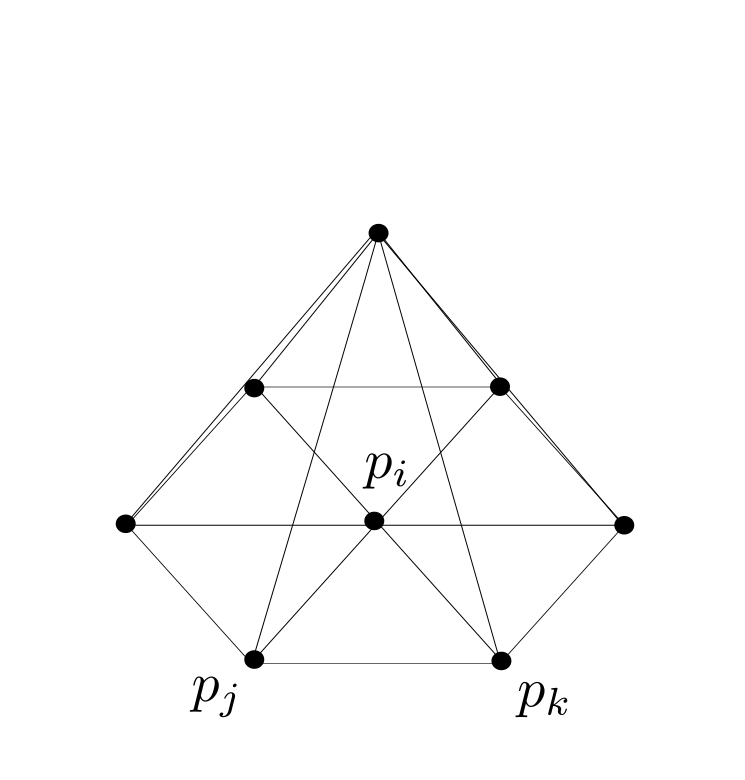
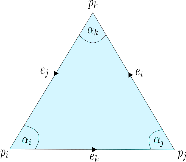
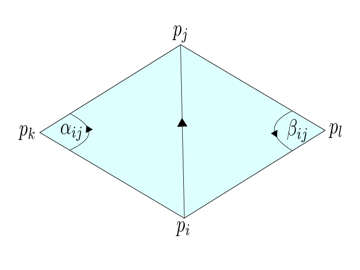
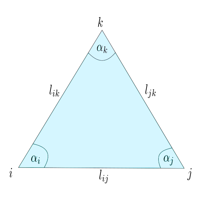
Note that every realization $p:V \rightarrow \mathbb{R}^3$ induces a metric on the underlying triangulated surface. On the other hand a triangulated surface with metric has several realization in $\mathbb{R}^3$, such that the metrics coincide. On a triangulated surface with metric every triangle has the structure of an euclidean triangle in $\mathbb{R}^2$, that allows us to interpolate $f:V\rightarrow \mathbb{R}$ to a piecewise affine function $\tilde{f}: C\left( \Sigma\right) \rightarrow \mathbb{R}$ and define the Dirichlet energy $E_D(f)$ as in the last lectures.

 In particular, we can define angles and area using the cosine theorem:
\[\cos(\alpha_i) = \frac{l_{jk}^2-l_{ji}^2-l_{ki}^2}{2l_{ki}l_{ij}}\]
By the triangle inequalities we obtain that $0 < \gamma <\pi$ and the angles are well defined. With $\sin(\alpha_i) = \sqrt{1-\cos(\alpha_i)^2}$ we can define the cotangents weights and the area of the triangle $\sigma = \{i,j,k\}$ :
\[A_{\sigma} = \frac{1}{2} \sin{(\alpha_i})l_{ij} l_{ki}.\]
For a realization $p$ of $\Sigma$ with vertex positions $p_i,p_j,p_k$ and edges $e_{ij} = p_j-p_i, \ldots $ we obtain for $\sigma = \{i,j,k\} \in F$:
\[A_{\sigma}(p) =  \frac{1}{2}\left| (p_j-p_i) \times (p_k-p_i) \right| = \frac{1}{2}\left| e_{ij} \times e_{ik}\right| = \frac{1}{2} \sin{(\alpha_i})\underbrace{|e_{ij}|}_{ =l_{ij}} \underbrace{|e_{ki}|}_{=l_{ki}},\]
and the total area is give by:
\[A (p) = \sum_{\sigma \in F} A_{\sigma}(p).\]

Definition: The following problem is the Plateau problem: Let $\Sigma$ be a triangulated surface with boundary and $q: V^{\partial} \rightarrow \mathbb{R}^3 $ a prescribed function. We are looking for a realization $p:V \rightarrow \mathbb{R}^3$ of $\Sigma$ such that:

1.  $\left. p \right|_{V^{\partial}} = q,$
2.  $ p$ has the smallest area among all realizations $ \tilde{p}$ of $\Sigma$, with $ \left. \tilde{p} \right|_{V^{\partial}} = q$.

In order to be able to solve the  Plateau problem we have to consider variations of $p$:

Definition: A variation of $p$ with constant boundary assigns to each vertex  $i \in V$ a curve $ t \mapsto p_i(t), $ $ t \in (- \epsilon ,\epsilon) ,$ such that:

1. $p_i(0) = p_i $ for all $i \in V.$
2. $p_j(t) = q_j $ for all $ t \in (- \epsilon ,\epsilon)$ if $j \in V^{\partial}$.

Definition: $p$ is called a minimal surface if it is a critical point of the area functional, i.e. :
\[\left. \frac{\partial}{\partial t} \right|_{t=0} A \left(p(t) \right) = 0,\]
for all variations of $p$ with constant boundary.

Lemma: $p$ is a minimal surface if and only if For each $i \in \overset{\circ}{V}$ and each curve $ t \mapsto p_i(t), $ $ t \in (- \epsilon ,\epsilon) $ we have:
\[\left. \frac{\partial}{\partial t} \right|_{t=0} A \left(p_i(t) \right) = \left. \frac{\partial}{\partial t} \right|_{t=0} \sum_{\sigma \in F \, \vert \, i \in \sigma} A_{\sigma} \left(p_i(t) \right) = 0.\]

I.e. $p$ is a critical point of the area functional with respect to all variations with constant boundary, if and only if it is a critical point for all those variations that only move one interior vertex.

Proof: $”\Rightarrow”:$ clear.
$”\Leftarrow:”$ Similar to the following fact from analysis:
All directional derivatives of a function $f: U \rightarrow \mathbb{R}, \quad U \subset \mathbb{R}^n$ vanish at $p \in U$ if and only if all partial derivatives of $f$ vanish at $p$.

$\square$

Theorem: $p$ is a minimal surface if and only if all tree components of $p$ are discrete harmonic functions with respect to the metric induced on $\Sigma$ by $p$.

Proof: piramid p_i
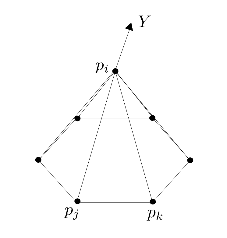
Fix $i \in \overset{\circ}{V}$ and let  $ t \mapsto p_i(t), $ $ t \in (- \epsilon ,\epsilon) $ be a variation, that only moves $p_i$ and $Y:= p_i'(o). $ Further we define $\hat{F} := \left\{ \{i,j,k\} \in F \big \vert \mbox{ positive oriented} \right\}$ to be the set of positive oriented triangles that contain the vertex $i$. We have to show that there holds:
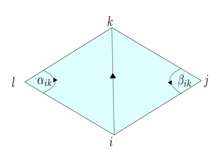
\begin{align}0=\left. \frac{\partial}{\partial t} \right|_{t=0} A \left(p_i(t) \right) &= \left. \frac{\partial}{\partial t} \right|_{t=0} \sum_{\{i,j,k\} \in \hat{F}} \left| (p_j-p_i(t)) \times (p_k-p_i(t))\right| \\&= \left. \frac{\partial}{\partial t} \right|_{t=0} \sum_{\{i,j,k\} \in \hat{F}} \left| e_{ij}(t) \times e_{ik}(t) \right|.\end{align}

Before we start with the proof remember these identities from analysis$\backslash$linear algebra

1.  For a function $t\rightarrow v(t) \in \mathbb{R}^3$ there holds:
\begin{align} |v|’=\frac{\langle v, v’ \rangle}{|v|} \end{align}
2. For $a,b,c,d \in \mathbb{R}^3$ we have:
\begin{align} \langle a\times b, c \times d \rangle = \det \left( \begin{matrix} \langle a,c \rangle & \langle a,d \rangle \\ \langle b,c \rangle\ &\langle b,d \rangle\ \end{matrix} \right) = \langle a,c \rangle\langle b,d \rangle-\langle a,d \rangle\langle b,c \rangle.\end{align}
With $e_{i,j} = p_j-p_i$ we get $\dot{e_{ij}}=-Y$ and can compute now the variation of the area functional:
\begin{align*} \left. \frac{\partial}{\partial t} \right|_{t=0} &A \left(p_i(t) \right) = \frac{1}{2} \sum_{\{i,j,k\} \in \hat{F}} \frac{\langle e_{ij} \times e_{ik} , -Y \times e_{ik} – e_{ij} \times Y \rangle}{|e_{ij} \times e_{jk}|} \\ &= \sum_{\{i,j,k\} \in \hat{F}} \frac{-\langle e_{ij} ,Y\rangle |e_{ik}|^2 + \langle e_{ik},Y\rangle \langle e_{ij},e_{ik} \rangle -\langle e_{ik} ,Y\rangle |e_{ij}|^2 + \langle e_{ij},Y\rangle \langle e_{ij},e_{ik}  \rangle}{2|e_{ij} \times e_{jk}|} \\ &= \bigl\langle Y ,\sum_{\{i,j,k\} \in \hat{F}} \frac{-e_{ij}|e_{ik}|^2-e_{ik}|e_{ij}|^2 + \langle e_{ij},e_{ik}  \rangle (e_{ij} + e_{ik})}{2|e_{ij} \times e_{jk}|}\bigr\rangle \\&= \bigl\langle Y ,\sum_{\{i,j,k\} \in \hat{F}} \frac{\left( -\langle e_{ik},e_{ik}  \rangle + \langle e_{ij},e_{ik}  \rangle\right) e_{ij}+\left( -\langle e_{ij},e_{ij}  \rangle + \langle e_{ij},e_{ik}  \rangle\right) e_{ik}}{2|e_{ij} \times e_{jk}|} \bigr\rangle.\end{align*}
With \[-\langle e_{ik},e_{ik}  \rangle + \langle e_{ij},e_{ik}  \rangle = \langle e_{ik},e_{ij} -e_{ik}\rangle =\langle e_{ik},e_{kj}  \rangle, \]
and
\[-\langle e_{ij},e_{ij}  \rangle + \langle e_{ij},e_{ik}  \rangle = \langle e_{ij},e_{ik} -e_{ij}\rangle = \langle e_{ij},e_{jk}  \rangle,\]
We have:
\[ \left. \frac{\partial}{\partial t} \right|_{t=0} A \left(p_i(t) \right) = \bigl\langle Y ,\sum_{\{i,j,k\} \in \hat{F}} \left( \frac{ \langle e_{ik},e_{kj}  \rangle e_{ij}}{2|e_{ij} \times e_{jk}|}  \right) + \sum_{\{i,j,k\} \in \hat{F}} \left( \frac{\langle e_{ij},e_{jk}  \rangle e_{ik}}{2|e_{ij} \times e_{jk}|}  \right) \bigr\rangle. \]

2trianglesijkl

In an earlier lecture  we showed that: $\cot(\beta_{ik}) = \frac{\langle -e_{ij},e_{jk}\rangle }{|e_{ij} \times e_{jk}|} $ and $ \cot(\alpha_{ik}) = \frac{\langle e_{il},e_{kl}\rangle }{|e_{ik} \times e_{il}|}. $

With an index shift in the first sum $(i,j,k) \rightarrow (i,k,l)$ we have now : \begin{align*} \left. \frac{\partial}{\partial t} \right|_{t=0} A \left(p_i(t) \right) & = \bigl\langle Y ,-\sum_{\{i,j,k\} \in \hat{F}} \frac{1}{2}\bigl( \cot(\beta_{ik}) + \cot(\alpha_{ik})  \bigr) e_{ik} \bigr\rangle \\ & = \bigl\langle Y , -\sum_{\{i,k\} \in \hat{E}} \frac{1}{2} \bigl( \cot(\beta_{ik}) + \cot(\alpha_{ik})  \bigr) (p_k – p_i) \bigr\rangle. \end{align*}

Since this has to hold for all variations $Y$ of $p_i$ and for all $i \in \overset{\circ}{V} $we finally get:
\[ \left. \frac{\partial}{\partial t} \right|_{t=0} A  \left(p(t) \right) =0 \Leftrightarrow  \sum_{\{i,k\} \in \hat{E}} \frac{1}{2} \bigl( \cot(\beta_{ik}) + \cot(\alpha_{ik})  \bigr) (p_k – p_i)=0 \quad \forall i \in \overset{\circ}{V}. \]

This means $p$ is an minimal surface if and only if all components of $p$ are harmonic with respect to the metric on $\Sigma$ induced by $p$.

$\square$

Posted in Lecture | Comments Off on Triangulated surfaces with metric and the Plateau problem

Dirichlet energy 2

Let $M = (V,E,F)$  be a triangulated domain in the plane where $V$ denotes the set of vertices, $E$ the set of edges and $F$ the set of triangles.  We consider the set of functions on the vertices  :
\begin{align*} \mathbb{R}^V:= \left\{ \begin{array}{c}  f : & V  \rightarrow \mathbb{R} \\  & i \mapsto f_i  \end{array}\right\}.\end{align*}
By interpolation to a piecewise linear function we get:  $\hat{f}: M \rightarrow \mathbb{R}$.
\[\mathbb{R}^V \overset{\mbox{interpol.}}{\rightarrow} W_{PL}:=\left\{ \hat{f}:M\rightarrow \mathbb{R} \, \big \vert \,\left. \hat{f}\right|_{\sigma} \mbox{ is affine for all } \sigma \in F\right\}.\]
In the last lecture the Dirichlet energy of  $ \hat{f} \in W_{PL}$ was defined as:
\[E_D(\hat{f}) = \frac{1}{2} \int_M \left| \mbox{grad} \, \tilde{f} \right|^2 = \frac{1}{4} \sum_{(i,j) \in \hat{E}} \left( \cot(\alpha_{ij}) + \cot{\beta_{ij}}\right) \left(f_i-f_j \right)^2. \]
$  E_D : W_{PL} \rightarrow \mathbb{R} $ is a quadratic form, which can be represented by matrix $A \in \mathbb{R}^{V \times V}:$
\[E_D(f) = \left(  f_1, \ldots , f_N \right) \left( \begin{array}{ccc} a_{11} & \ldots &  a_{1N} \\ \vdots & \ddots & \vdots \\ a_{N1} & \ldots & a_{NN} \end{array} \right) \left( \begin{array}{ccc} f_1 \\ \vdots \\ f_N \end{array} \right),\]
where $N:=|V|$ and
\[a_{ij}:=\left\{ \begin{array}{rcl}
-\frac{1}{4}\left( \cot(\alpha_{ij}) + \cot{\beta_{ij}} \right) & \mbox{for}
& i\neq j, \,\{i,j\} \in E, \\  \frac{1}{4} \sum_{(i,k) \in \hat{E}} \left(\cot(\alpha_{ik}) + \cot{\beta_{ik}} \right) & \mbox{for} & i=j, \\ 0 & \mbox{else}. &
\end{array}\right.
\]
One can easily check that: $A\left( \begin{array}{c} 1 \\ \vdots \\1\end{array}\right)=0$ and even further there holds: $\mbox{ker } A = \mathbb{R}\left( \begin{array}{c} 1 \\ \vdots \\1\end{array}\right).$

In order to get a better understanding of the Dirichlet energy we recap some facts on quadratic forms.
There is a natural relation between symmetric bilinear forms and quadratic forms:

Proposition: Let $W$ be a vectorspace and $b:W \times W \rightarrow \mathbb{R}$ a bilinear symmetric form then
\begin{align*} q: W \rightarrow \mathbb{R}, \\ q(w):= b(w,w),\end{align*}
is the corresponding quadratic form. $b$ is completely determined by $q$.

Proof: \begin{align*} & q(w_1+w_2) = b(w_1+w_2,w_1+w_2)=q(w_1) + 2b(w_1,w_2) + q(w_2), \\ \Rightarrow \quad \quad & b(w_1,w_2) = \frac{1}{2} \left(q(w_1+w_2) – q(w_1) – q(w_2).\right)\end{align*}

$\square$

For a vectorspace $W$ the dualspace is defined as $W^{\ast}:= \left\{ w^{\ast}: W \rightarrow \mathbb{R} \, \big \vert \,w^{\ast} \mbox{ is linear }\right\}.$ For a basis of $W$ $\left\{w_1, \ldots ,w_n \right\}$ the corresponding dual basis of $W^{\ast}$ $\left\{w_1^{\ast}, \ldots ,w_n^{\ast} \right\}$ is defined by:
\[w_i^{\ast}(w_j) = \delta_{ij}.\]
Note that there is a natural identification of $W^{\ast \ast}$ and $W$, i.e. the dual space of the dual space is the original space.
For a linear map $A:W \rightarrow V$ between vectorspaces $W,V$ the adjoint map is defined as:
\begin{align*}A^{\ast} : V^{\ast} &\rightarrow W^{\ast} \\ \left( A^{\ast}v^{\ast}\right)(w) & := v^{\ast}\left( Aw\right) \quad \quad \forall v^{\ast} \in V^{\ast}\mbox{ and } \forall w \in W.\end{align*}

If $b: W \times W \rightarrow \mathbb{R}$  is a bilinear form, we can define a map $A: W \rightarrow W^{\ast}$ by:
\[\left(Aw_1\right)(w_2):= b(w_1,w_2).\]
Conversely a  map $A: W \rightarrow W^{\ast}$ defines a bilinear form on $W$. If the bilinear form $b$ is non degenerated $A$ is an isomorphism. In this case $b$ gives us an identification of elements of $W$ and $W^{\ast}.$ A typical example is given by an euclidean vectorspace $\left( W,\langle \cdot , \cdot \rangle \right)$. There we can identify an element $w \in W$ with $w^{\ast} \in W^{\ast}$ by:
\[w^{\ast} = \langle w , \cdot \rangle. \]

Proposition: With the identification above we have: $b: W \times W \rightarrow \mathbb{R}$ is symmetric if and only if $A: W \rightarrow W^{\ast}$ is self-adjoint.

Proof: First note that for $A: W \rightarrow W^{\ast}$ we have $A^{\ast}: \underbrace{W^{\ast \ast}}_{= W} \rightarrow W^{\ast}.$
\[b(w_1,w_2) = \left(Aw_1\right)(w_2) = \underbrace{w_2}_{\in W^{\ast \ast}}\left( Aw_1\right) = \left( A^{\ast}w_2\right)(w_1)\]
Therefore we get: \[b(w_1,w_2)=b(w_2,w_1) \Leftrightarrow A^{\ast} = A.\]

$\square$

Now lets get back to the Dirichlet energy. The quadratic form $E_D$ on $W_{PL}$ can be identified with a symmetric bilinear map $\tilde{E_D}: W_{PL} \times W_{PL} \rightarrow \mathbb{R}$, which again corresponds to linear map $\hat{E_D} : W_{PL} \rightarrow W_{PL} ^{\ast}$. Together with the interpolation map we obtain the following diagram:
\[\begin{array}{lcl} W_{PL} & \overset{\hat{E_D}}{\longrightarrow}  & W_{PL}^{\ast} \\ \uparrow \mbox{interpol.} &  & \downarrow \mbox{interpol.}^{\ast} \\ \mathbb{R}^V & \overset{A}{\longrightarrow} & \mathbb{R}^{V\ast} \end{array}  \]

If $\overset{\circ}{V}$ denotes the set of interior vertices and $V^{\partial}$ the one of boundary vertices we can give a discrete analog of the Dirichlet boundary problem in the following way:

Theorem: Given $g:V^{\partial} \rightarrow \mathbb{R}$ there is a unique $f:V \rightarrow \mathbb{R}$ such that:
\[\left\{ \begin{array}{ll} \left(A f \right)_i = 0 \quad \forall i \in \overset{\circ}{V}, \\ \left. f\right|_{V^{\partial}} = g.\end{array} \right.\]

A function $f:V \rightarrow \mathbb{R}$ that solves the above Dirichlet problem is called harmonic.

Posted in Lecture | Comments Off on Dirichlet energy 2

Gradient and Dirichlet energy on triangulated domains.

Let $M$ be a triangulated domain with the functionspace:
\[W_{PL}:=\bigl\{f:M\rightarrow\mathbb{R}\,\bigl\vert\bigr.\,\,\,\left. f\right|_{T_{\sigma}} \mbox{ is affine for all } \sigma \in \Sigma_2 \bigr\}.\]
On the interior of each triangle $T_{\sigma}$ in $M$ the gradient of a function $g \in W$ is well defined and constant. We will derive a nice formula to compute $\left. \mbox{grad}\;g \right|_{T_{\sigma}}$.

Theorem 1: Let $T \subset \mathbb{R}^2$ be a non degenerated triangle with vertices $p_i,p_j,p_k$ and edges $e_i :=p_k-p_j$, $e_j :=p_i-p_k$, $e_k :=p_j-p_i$. For an affine function $g:T\rightarrow \mathbb{R}$ we define $g_i:=g(p_i)$, $g_j:=g(p_j)$, $g_k:=g(p_k)$. Then there holds:
\[\mbox{grad}\, g = \frac{1}{2A}J\bigl( g_i e_i+g_j e_j+ g_k e_k\bigr),\]
where $A:=\frac{1}{2}\mbox{det}(e_i,e_j) = \frac{1}{2} \langle Je_i,e_j \rangle=\frac{1}{2}\langle Je_j,e_k \rangle=\frac{1}{2}\langle Je_k,e_i \rangle,$ denotes the area of $T$ and $J$ the usual $90$ degree rotation in the plan.

Proof: In order to compute $\mbox{grad}\, g$ consider the curvepath6075-9
\begin{align*} & \gamma : [0,1] \rightarrow \mathbb{R}^2,\\ & \gamma(t)  :=p_j + te_i. \end{align*}
The composition of $g$ and $\gamma$ is given by: $\left( g\circ \gamma\right)(t) = g_j + t\left( g_k – g_j\right)$. Taking the derivative direct and with respect to the product rule we get:
\[g_k -g_j = \left( g\circ \gamma\right)'(t) = g’\left(\gamma(t)\right) \cdot\gamma'(t) = \langle \mbox{grad} \, g, \gamma'(t) \rangle = \langle \mbox{grad} \, g,e_i \rangle. \]
On the other hand we have:
\begin{align*}\bigl\langle\frac{1}{2A}J\left( g_i e_i+g_j e_j+ g_k e_k\right),e_i \bigr\rangle & = \frac{1}{2A} \bigl(g_i \underbrace{\langle Je_i,e_i\rangle }_{=0} + g_j \underbrace{\langle Je_j,e_i\rangle}_{=-2A} + g_k \underbrace{\langle Je_k,e_i\rangle}_{= 2A}\bigr) \\ &= g_k -g_j.\end{align*}
And therfore:
\[\bigl\langle\frac{1}{2A}J\left( g_i e_i+g_j e_j+ g_k e_k\right),e_i \bigr\rangle = \bigl\langle \mbox{grad} \, g,e_i \bigr\rangle.\]
A cyclic permutation of $i,j,k$  gives us:
\[\bigl\langle\frac{1}{2A}J\left( g_i e_i+g_j e_j+ g_k e_k\right),e_j \bigr\rangle = \bigl\langle \mbox{grad} \, g,e_j \bigr\rangle,\]
and we obtain the desired result \[\mbox{grad}\, g = \frac{1}{2A}J\bigl( g_i e_i+g_j e_j+ g_k e_k\bigr).\]

$\square$

Definition: For $g \in W_{PL}$ the Dirichlet energy is defined as:
\[E_D(g) := \frac{1}{2} \int_M \left| \mbox{grad} \, g \right|^2.\]

Theorem 2: We use the same notation as in theorem 1. Additionally let $\alpha_i,\,\alpha_j,\, \alpha_k$ denote the angles of the triangle at the vertices $p_i, \, p_j, \, p_k$ respectively. Then there holds:
\[ \int_T \left| \mbox{grad} \, g \right|^2 = \frac{1}{2}\bigl( \cot (\alpha_i) (g_j-g_k) ^2 + \cot (\alpha_j) (g_k-g_i) ^2 + \cot (\alpha_k) (g_i-g_j) ^2\bigr).\]

Proof: \begin{multline}\int_T \left| \mbox{grad} \, g \right|^2 = \int_T \langle \frac{1}{2A}J\left( g_i e_i+g_j e_j+ g_k e_k\right), \frac{1}{2A}J\left( g_i e_i+g_j e_j+ g_k e_k\right) \rangle \\ =\frac{A}{4 A^2} \Bigl(\Bigr. g_i^2 |e_i|^2 +  g_j^2 |e_j|^2 + g_k^2 |e_k|^2 + 2g_ig_j \langle e_i,e_j \rangle + 2g_jg_j \langle e_j,e_k \rangle + 2g_kg_i \langle e_k,e_i \rangle \Bigl)\Bigr..  \end{multline}
On the other hand we have:
\begin{align}\frac{-1}{4A} \bigl(\bigr. \left( g_i -g_j\right)^2 & \langle e_i, e_j \rangle +\left( g_j -g_k\right)^2 \langle e_j, e_k \rangle +\left( g_k -g_i\right)^2 \langle e_k, e_i \rangle \bigl)\bigr. \\ &= \frac{-1}{4A} \bigl(\bigr. g_i^2 \langle e_i,\underbrace{e_j + e_k}_{= – e_i}\rangle -2g_ig_j\langle e_i,e_j \rangle + g_j^2 \langle e_j, \underbrace{e_i + e_k}_{= – e_j}\rangle \\ &\quad\quad\quad -2g_kg_j\langle e_k,e_j \rangle +g_k^2 \langle e_k, \underbrace{e_j + e_i}_{=- e_k}\rangle -2g_ig_k\langle e_i,e_k \rangle \bigl)\bigr. \\ &= \frac{1}{4 A} \bigl(\bigr. g_i^2 |e_i|^2 +  g_j^2 |e_j|^2 + g_k^2 |e_k|^2 \\ &\quad\quad\quad+ 2g_ig_j \langle e_i,e_j \rangle + 2g_jg_j \langle e_j,e_k \rangle + 2g_kg_i \langle e_k,e_i \rangle \bigl)\bigr. \\ & = \int_T \left| \mbox{grad} \, g \right|^2.\end{align}
With \begin{align*}\langle e_i,e_j \rangle & = -\cos (\alpha_k) |e_i||e_j|,\\2A = \frac{1}{2}\mbox{det}(e_i,e_j) & = \frac{1}{2} \langle Je_i,e_j \rangle
= \sin(\alpha_k) |e_i||e_j|.\end{align*}
We have:
\[\cot(\alpha_k) = \frac{-\langle e_i,e_j \rangle}{2A}.\]
And therefore we obtain for the Dirichlet energy of $g$ on $T$:
\[ \int_T \left| \mbox{grad} \, g \right|^2 = \frac{1}{2}\bigl( \cot (\alpha_i) (g_j-g_k) ^2 + \cot (\alpha_j) (g_k-g_i) ^2 + \cot (\alpha_k) (g_i-g_j) ^2\bigr).\]

$\square$

Corollary: The Dirichlet energy of $g \in W_{PL}$ is given by :
\[E_D(g) = \frac{1}{4} \sum_{\sigma = \{i,j,k\} \in \Sigma_2}  \cot (\alpha_i) (g_j-g_k) ^2 + \cot (\alpha_j) (g_k-g_i) ^2 + \cot (\alpha_k) (g_i-g_j) ^2.\]

 2triangles

If $E:= \left\{ \{i,j\} \in \Sigma\right\}$ denotes the set of edges and $\tilde{E}:= \left\{ (i,j) \in V \times V\, \big \vert \{i,j\} \in \Sigma\right\}$ the set of oriented edges, we choose $\hat{E} \subset \tilde{E}$ such that:

1)  $E = \left\{ \{i,j\} \subset V \big \vert (i,j) \in \hat{E}\right\}$,
2)  $(i,j) \in \hat{E} \rightarrow (j,i) \notin \hat{E}.$

I.e. for every edges we choose oneoriented one. For every $(i,j) \in \hat{E}$ let $\alpha_{ij}$ denote the angle of the opposite vertex to the left and $\beta_{ij}$ the one the opposite vertex to the right. Then we can write the Derichlet energy in the following form:
\[E_D(g) = \frac{1}{4} \sum_{(i,j) \in \hat{E}} \left( \cot(\alpha_{ij}) + \cot{\beta_{ij}}\right) \left(g_i-g_j \right)^2, \]
where we set the cotangent weights zero if the corresponding vertex does not exist because $(i,j)$ is an boundary edge.

Posted in Lecture | Comments Off on Gradient and Dirichlet energy on triangulated domains.

Triangulated surfaces and domains

We want to derive a discrete version of the laplace operator defined on triangulated surfaces. At first we will define what a triangulated surface with and without  boundary is,  and consider triangulated domains of $\mathbb{R}^2$ as an important example.

Let $\Sigma$ be a two dimensional simplicial complex and let $V$ denote its set of vertices. For $i \in V$ the “vertex-star” around $i$ is defined as:
\[S_i := \left\{ j \in V\, \big \vert \, j \neq i, \, \{i,j\} \in \Sigma \right\}.\]The link of a vertex $i \in V$ is a graph $G_i$ given by:
\[G_i := \left\{ \{j,k\}\subset S_i \,\big \vert \, j \neq k, \, \{i,j,k\} \in \Sigma\right\}.\]

Definition: A triangulated surface with boundary is a two dimensional simplicial complex $\Sigma$ with the following properties:
1) Each edge is contained in exactly one or two triangles.
2) For each vertex $i \in V$ the corresponding link $G_i$ is connected.

A vertex of a link $G_i$ has either one or two edges. In a triangulated surface with boundary all links $G_i$ are  connected  thus they are either a discrete interval or a discrete circle. In the first case the corresponding vertex $i$ is called a boundary vertex in the second case it is called an interior vertex. Also the edges of an triangulated surface split in two groups. The one that are contained in only one triangle are the boundary edges, the one that lie in two triangles are interior edges. The set of all boundary vertices and edges of an triangulated surface with boundary is a graph, called the boundary of $\Sigma$ and will be denoted with $\partial \Sigma$.
The boundary is either empty or the union of discrete circles. If the boundary is empty $\Sigma $ is called a triangulated surface.

Definition: A triangulated domain $M$ in $\mathbb{R}^2$ is a triangulated surface with boundary $\Sigma$ together with an assignment $p:V\rightarrow \mathbb{R}^2$ such that its piecewise linear extension $\tilde{p}: C(\Sigma) \rightarrow \mathbb{R}^2$ is injective. Then $M$ is given by the following disjoint union:
\[M= \bigcup_{S \in \Sigma}^{\circ} \tilde{p} \left(\overset{\circ}{C(S)}\right).\]

Here $\tilde{p} \left(\overset{\circ}{C(S)}\right)$ denotes the interior of the affine realization of the simplex $S$. For a triangle this is the triangle minus its edges, for an edge it is the edge minus its vertices and the interior of a point is just the point it self.

For $\sigma \in \Sigma_2 $ let $T_{\sigma}:=\tilde{p}\left(C(\sigma)\right)$ denote the corresponding triangle in $M \subset \mathbb{R}^2$  and for $i \in V$, $p_i:=\tilde{p}\left(\delta(i) \right)$   the corresponding point .

On a triangulated domain  $M \subset \mathbb{R}^2$ we consider the following set of functions:
\[W:=\left\{ f:M\rightarrow \mathbb{R} \, \big \vert \,\left. f\right|_{T_{\sigma}} \mbox{ is affine for all } \sigma \in \Sigma_2, \, \left. f\right|_{\partial M}=0 \right\}\]
We can equip $W$ with the usual scalar-product:
\begin{align*}\langle\!\langle\cdot, \cdot \rangle\!\rangle &: W\times W \rightarrow \mathbb{R}, \\ \langle\!\langle f, g \rangle\!\rangle & := \int_M fg.\end{align*}
On the interior of each triangle $T_{\sigma}$, $f \in W$ is a differentiable function with constant derivative. Therefore, for all $\sigma \in \Sigma_2$ there exist $X_{\sigma} \in \mathbb{R}^2$ such that $\mbox{grad}\,f(p) = X_{\sigma}$ for all $p \in \overset{\circ}{T_{\sigma}}$. More general we define the set of vector fields on $M$:
\[VF(M):= \left\{X:\bigcup_{\overset{\circ}{T_{\sigma}},\,\sigma \in \Sigma_2}\rightarrow \mathbb{R}^2 \,\bigg \vert \,\left. X\right|_{\overset{\circ}{T_{\sigma}}} = X_{\sigma}=\mbox{constant, for all } \sigma\in \Sigma_2\right\}\]
Also on $VF(M)$ we can define a scalar product:
\begin{align*}\langle\!\langle\cdot, \cdot \rangle\!\rangle &: VF(M)\times VF(M) \rightarrow \mathbb{R}, \\ \langle\!\langle X, Y \rangle\!\rangle & := \sum_{ \sigma\in \Sigma_2}\langle X_{ \sigma},Y_{ \sigma}\rangle A_{ \sigma},\end{align*}
where $A_{ \sigma}$ denotes the area of $T_{\sigma}.$

Let $\overset{\circ}{V}$ denote the set of interior vertices of $\Sigma$ and $N:=\left|\overset{\circ}{V}\right|$ the number of interior vertices. A function $f \in W$ is completely determined by its values $f_i:= f(p_i)$ at the interior vertices of the triangulation. In deed, $W$ is a $N$ dimensional vectorspace with basis $\left\{\phi_i\right\}$, where $\phi_i \in W$ is defined by $\phi_i(p_j):=\delta_{ij}.$ The $\phi_i$ are often called “hat-function” and there holds:
\[f = \sum_{i \in \overset{\circ}{V}} f_i \phi_i.\]
Thus in order to compute the scalar product of arbitrary functions $f,g \in W$ we just need to know the values:
\[b_{ij}:=\langle\!\langle\phi_i, \phi_j \rangle\!\rangle.\]
For $\{i,j\}\notin \Sigma$  we have $b_{ij}:=\langle\!\langle\phi_i, \phi_j \rangle\!\rangle=0.$

In order to compute the non zero elements consider the domain \[D:= \left\{(s,t) \in \mathbb{R}^2 \, \big \vert \, 0\leq s,t,s+t \leq 1\right\},\]
and for each triangle $T_{\sigma}$ with vertices $p_i,p_j,p_k$ and edges $e_{k}:= p_j – p_i$, $e_{i}:= p_k – p_j$, $e_{j}:= p_i – p_k$ the following parametrization:
\begin{align*}\Phi &:D \rightarrow T_{\sigma} \subset \mathbb{R}^2, \\ \Phi(s,t) &:= p_i + t e_{k} – s e_{j}.\end{align*}
$\Phi$ is bijective and we have:
\[\mbox{det}\left( \Phi’\right) = \mbox{det}\left( e_{k},-e_{j}\right) = 2A_{\sigma}.\]
Now we can compute $\langle\!\langle\phi_i, \phi_i \rangle\!\rangle$:
\begin{align*}\int_{T_{\sigma}} \phi_i^2 & = \int_D \left(\phi_i \circ \Phi\right)^2 \left| \,\mbox{det}\left( \Phi’\right)\right|  \\ &= \int_D (1-s-t)^2 2A_{\sigma} \,ds dt \\ &= 2A_{\sigma} \int_0^1\int_0^{1-t} (1-s-t)^2 ds dt \\ &= 2A_{\sigma} \int_0^1 \frac{-1}{3} \left. (1-s-t)^3\right|_0^{1-t}  dt \\ &= 2A_{\sigma} \int_0^1 \frac{1}{3} (1-t)^3 dt\\ & = \frac{A_{\sigma}}{6}.
\end{align*}
Summation over all triangles that contain the vertex $i$ gives us the result:

\[b_{ii} = \langle\!\langle\phi_i, \phi_i \rangle\!\rangle = \int_M \phi_i^2 =\sum_{\sigma \,\vert \, i \in\sigma }\int_{T_{\sigma}} \phi_i^2 = \frac{1}{6} \sum_{\sigma \,\vert \, i \in\sigma }A_{\sigma}.\]
To every vertex $i \in V$ we can assign an area
\[A_i:=\frac{1}{3} \sum_{\sigma \,\vert \, i \in\sigma }A_{\sigma},\] and obtain  $\langle\!\langle\phi_i, \phi_i \rangle\!\rangle = \frac{1}{2} A_i.$ Using $\left(\phi_j \circ \Phi\right)(s,t) = s$ and $\left(\phi_k \circ \Phi\right)(s,t) = t$ we obtain the analog result for $\langle\!\langle\phi_j, \phi_k \rangle\!\rangle$:
\begin{align*}\int_{T_{\sigma}} \phi_j \phi_k & = \int_D \left(\phi_j \circ \Phi\right) \left(\phi_k \circ \Phi\right) \left| \,\mbox{det}\left( \Phi’\right)\right| \\ & = 2A_{\sigma}\int_D st \, ds dt \\ &= 2A_{\sigma} \int_0^1\int_0^{1-t} st \, ds dt \\ & = A_{\sigma} \int_0^1 \left. ts^2\right|_0^{1-t}  dt \\ &= A_{\sigma} \int_0^1 t^3-2t^2+t  \, dt \\ &= \frac{A_{\sigma}}{12}.
\end{align*}
And again we get the result by summation over the two triangles that contain $j$ and $k$:
\[b_{jk} = \langle\!\langle\phi_j, \phi_k \rangle\!\rangle = \frac{1}{12} \sum_{\sigma \,\vert \, k,j \in\sigma }A_{\sigma}.\]
The scalar product of two functions $f = \sum_{i \in \overset{\circ}{V}} f_i \phi_i, \quad g = \sum_{i \in \overset{\circ}{V}} g_i \phi_i$ can now be computed in the following way:
\[\langle\!\langle f, g \rangle\!\rangle = \sum_{i,j \in \overset{\circ}{V}} f_i g_j \langle\!\langle\phi_i, \phi_j \rangle\!\rangle = \sum_{i,j \in \overset{\circ}{V}} f_i g_j b_{ij}.\]

Posted in Lecture | Comments Off on Triangulated surfaces and domains

Laplace operator 1

Let $M \subset \mathbb{R}^2$ be a domain with smooth boundary $\partial M$ and outpointing normal vector field $N$. For a smooth function $f \in C^{\infty}(M,\mathbb{R})$ the gradient vector field $\mbox{grad} \, f :M \rightarrow \mathbb{R}^2$ is defined as :
\[ \mbox{grad} \, f := \left( \begin{array}{c} \frac{\partial f}{\partial x} \\ \frac{\partial f}{\partial y} \end{array} \right)  = \left( f’\right)^t. \]
For a vector field $v:M \rightarrow \mathbb{R}^2$ the divergence is given by:
\[\mbox{div} \, v := \frac{\partial v_1}{\partial x} +\frac{\partial v_2}{\partial y}.\]
Taking this together we can define the laplace operator $\Delta : C^{\infty}(M,\mathbb{R})\rightarrow C^{\infty}(M,\mathbb{R})$:
\[\Delta \,f := \mbox{div} \, \mbox{grad}\, f = \frac{\partial^2 f}{\partial x^2} +\frac{\partial^2 f}{\partial y^2}.\]
The laplace operator plays an important role in physics and geometry. A typical problem from physics is the following called Dirichlet boundary problem: Given $g \in C^{\infty}(\partial M,\mathbb{R})$ find $f \in C^{\infty}(M,\mathbb{R})$ such that:
\[\left\{ \begin{array}{cc} \Delta \, f = 0 \\  \left. f\right|_{\partial M} = g.\end{array} \right.\]
If $f$ is a temperature distribution on $M$ and $g$ is the prescribed temperature on the boundary, then $f$ has to solve the heat equation: $\dot{f} = \Delta \, f.$ For a stationary temperature distribution there holds $\dot{f}=0$ and we obtain the above Dirichlet boundary problem.

Theorem:
1) Given $g \in C^{\infty}(\partial M,\mathbb{R})$ and $d \in C^{\infty}(M,\mathbb{R})$, then there is a unique $f \in C^{\infty}(M,\mathbb{R})$ such that: \[\left\{ \begin{array}{cc} \Delta \, f = d \\ \left. f\right|_{\partial M} = g.\end{array} \right.\]
2) If $d=0$ and $f$ is a solution of the corresponding Dirichlet boundary problem, then $f$ minimizes the Dirichlet energy \[ E_D(f):=\frac{1}{2}\int_M \left|\mbox{grad}\,f\right|^2,\] among all the functions $h \in C^{\infty}(M,\mathbb{R})$ with $\left. h\right|_{\partial M} = g.$

Proof:
1) The proof of the existence of $f$ is hard and can be found in some good books about PDE’s. We only proof the uniqueness of $f$.
Suppose there exists $f,\tilde{f} \in C^{\infty}(M,\mathbb{R})$ with: \( \Delta \, f =  \Delta \,\tilde{f} =0\) and \(\left. f\right|_{\partial M} =\left. \tilde{f}\right|_{\partial M} =g\), then $u:= \tilde{f} -f$ solves:
\[\left\{ \begin{array}{cc} \Delta \, u = 0 \\\left. u\right|_{\partial M} = 0.\end{array} \right.\]Now we consider the vector field $X:= u\, \mbox{grad} \,u$. For the divergence of $X$ we get:
\[ \mbox{div}\,X = \mbox{div} (u\, \mbox{grad} \,u) =\langle \mbox{grad}\,u, \mbox{grad} \,u\rangle\ + u\, \mbox{div}\, \mbox{grad} \, u =  \langle \mbox{grad}\,u, \mbox{grad} \,u\rangle\ + u \Delta \,u.\]
Using the fact that $X$ vanishes on the boundary and applying the divergence theorem we obtain:
\[0=\int_{\partial M}\langle X, N\rangle = \int_M \mbox{div}\,X = \int_M \langle \mbox{grad}\,u, \mbox{grad} \,u\rangle\ + u \Delta \,u = \int_M \left|\mbox{grad}\,u\right|^2.\]
Therefore, we have  $\mbox{grad} \,u=0$ on the whole of $M$ and $u$ is locally constant. Due to the fact that, $\left. u\right|_{\partial M} = 0$ $u$ is identically zero and therefore $f$ is unique.

2)Let $f$ be the unique solution of the Dirichlet boundary problem $\Delta \,f =0, \quad\left. f\right|_{\partial M} =g$ and $h$ an arbitrary smooth function with  $\left. h\right|_{\partial M} =g$. For $u:=h-f$ there holds $\left. u\right|_{\partial M} =0$ and we get:
\[\int_M \left|\mbox{grad},h\right|^2=\int_M \left|\mbox{grad}\,f+u\right|^2=\int_M \left|\mbox{grad}\,f\right|^2+ 2 \int_M \langle \mbox{grad}\,f ,\mbox{grad}\,u \rangle + \int_M \left|\mbox{grad}\,u\right|^2.\]
Using the usual product rule:
\[\mbox{div}(u\,\mbox{grad}\,f ) = \langle \mbox{grad}\,f ,\mbox{grad}\,u \rangle + u\, \Delta\,f, \] and the divergence theorem we obtain:
\begin{align*}2E_D(h)=\int_M \left|\mbox{grad}\,h\right|^2 &=\int_M \left|\mbox{grad}\,f\right|^2+ 2 \int_M \mbox{div}(u\,\mbox{grad}\,f ) -u\, \underbrace{\Delta\,f}_{=0}  + \int_M \underbrace{\left|\mbox{grad}\,u\right|^2}_{\geq 0}\\ &\geq \int_M \left|\mbox{grad}\,f\right|^2 + \int_{\partial M} \underbrace{u\langle \mbox{grad}\, f,N \rangle}_{=0}\\ &= \int_M \left|\mbox{grad}\,f\right|^2 = 2E_D(f).\end{align*}

$\square$

Let us now consider the space of smooth functions on $M$ that vanish at the boundary: \[V:= \left\{f \in  C^{\infty}(M,\mathbb{R}) \, \big\vert \, \left. f\right|_{\partial M}=0 \right\}\]
We can equip  $V$ with two  scalar products $\langle\!\langle \cdot, \cdot \rangle\!\rangle , \, \langle\!\langle\cdot, \cdot \rangle\!\rangle_D :V\times V \rightarrow \mathbb{R},$
\begin{align*}\langle\!\langle f, g\rangle\!\rangle &:=\int_M fg, \\ \langle\!\langle f, g\rangle\!\rangle_D & := \int_M \langle \mbox{grad}\,f ,\mbox{grad}\,g \rangle.\end{align*}
To see that $\langle\!\langle\cdot, \cdot \rangle\!\rangle_D$  is really a scalar product on $V$ one has to check that it is positive definite (symmetry and bi-linearity are obvious).
\begin{align*} & 0=\langle\!\langle f, f\rangle\!\rangle_D  = \int_M \left|\mbox{grad}\,f\right|^2 \\  \Leftrightarrow & \quad \left|\mbox{grad}\,f\right| = 0  \end{align*}
Therefore, $f$ is locally constant. With $\left. f\right|_{\partial M}=0$ one has $f=0$.

Propositon: On V the laplace operator is self adjoint, i.e. $\langle\!\langle \Delta \,f, g\rangle\!\rangle = \langle\!\langle f, \Delta \, g\rangle\!\rangle$ and  there holds: \[\langle\!\langle \Delta \,f, g\rangle\!\rangle =-\langle\!\langle f, g\rangle\!\rangle_D .\]

Proof: \begin{align*} \langle\!\langle \Delta \,f, g\rangle\!\rangle & = \int_M g\, \mbox{div} \, \mbox{grad}\, f  = \int_M  \mbox{div} (g \, \mbox{grad}\, f ) \,- \langle \mbox{grad} \,f ,\mbox{grad} \,g \rangle \\ & = \underbrace{\int_{\partial M} f \langle \mbox{grad} \,g , N \rangle}_{=0}  – \int_M \langle \mbox{grad} \,f ,\mbox{grad}\,g \rangle  \\ &=\,-  \langle\!\langle f, g\rangle\!\rangle_D \\ &= \,- \langle\!\langle g, f\rangle\!\rangle_D \\ & \,\, \vdots \\& =\langle\!\langle f, \Delta \, g\rangle\!\rangle.\end{align*}

$\square$

Posted in Lecture | Comments Off on Laplace operator 1

Tutorial 10 – Discrete minimal surfaces

In the lecture we have defined what we mean by a discrete minimal surface. The goal of this tutorial is to visualize such minimal surfaces.

Let \(\mathrm M\) be a discrete surface with boundary and let \(V, E, F\) denote the set of vertices, (unoriented) edges and faces. Once we have a discrete metric, i.e. a map \(\ell \colon E \to (0,\infty)\) such that the triangle inequalities hold,\[\ell_{ij} \leq \ell_{ik}+ \ell_{kj}, \quad \ell_{jk}\leq \ell_{ji} + \ell_{ik},\quad \ell_{ki} \leq \ell_{kj}+ \ell_{ji},\quad \textit{ for each }\sigma = \{i,j,k\},\]we can define the corresponding discrete Dirichlet energy \(E_D^\ell\):\[E_D^\ell (f) = \sum_{ij\in \tilde E} \omega_{ij}^\ell\,(f_j-f_i)^2,\quad \omega^\ell_{ij} = \tfrac{1}{2}(\cot \alpha_{ij} + \cot\beta_{ij}).\]Here \(\tilde E\) denote the positively oriented edges. Certainly the angles and thus the cotangent weights depend on the metric \(\ell\).

In particular, each map \(f\colon \mathrm M \to \mathbb R^3\), which maps thecombinatoric triangles to a non-degenerate triangles in \(\mathbb R^3\), yields an induced discrete metric,\[\ell_{ij} = |p_j – p_i|.\]We have seen in the lecture that a surface is minimal, i.e. a critical point of the area functional under all variations fixing the boundary, if and only if it solves the Dirichlet problem (with respect to its induced metric): For each interior vertex \(i\in\mathring V\) we have\[-\tfrac{1}{2}\sum_{\{i,j\}\in E}\,\omega_{ij}^\ell f_i +\tfrac{1}{2}\sum_{\{i,j\}\in E}\,\omega_{ij}^\ell f_j = 0,\]where \(\ell\) denotes the metric induced by \(f\).

Unfortunately, unlike the Dirichlet problem, this is a non-linear problem – the cotangent weights depend on \(\ell\) in a complicated way. Though, fortunately, we can solve it in many cases by iteratively solving a Dirichlet problem (here a paper that describes this). Since we know how to solve the Dirichlet problem we can implement this method without any effort.

network_plateauproblem

The network above visualizes Plateau’s problem: Given a space curve \(\gamma\) compute a minimal disk with boundary \(\gamma\). Actually this corresponds to a soap film spanned into a wire.

In the discrete setup we start with some discrete space, say generated by a curve node (probably followed by a resample node), which we then stick into a remesh node to get a reasonably triangulated disk spanned in. Then we can apply the iteration to this input. Below one possible result:

plateau2_

For rendering we used here the following texture in the mantra surface material. To generate texture coordinates one can use the nodes uvunwrap or uvtexture.

The algorithm is not restricted to disks. We can stick in any surface we want. Another nice example is e.g. obtained by starting with a cylinder of revolution. Here the minimal surface becomes a part of a catenoid or, if the cylinder’s height becomes to large, it degenerates to a pair of flat disks (connected by a straight line). In the picture below the last two circles are already too far apart – the surface starts to splits into two parts.

cylinders

As a last example we can start with the unit sphere into which we cut several holes. If we want nice symmetries we could use a platonic solid node to copy smaller spheres to the vertex positions of e.g. an octahedron. The area enclosed by the smaller spheres we then subtract from the unit sphere with help of a cookie node. If we run then the algorithm on this input we end up with nice symmetric minimal surface. For a certain radius of the holes the surface is close to the Schwarz P surface.

schwarzP_

Again one can observe the same effect as for the cylinder – if the holes get to small the minimal surface degenerates to several spheres connected to the origin.

Homework (due 12/14 July). Build a network that computes from a given discrete surface with boundary a minimal surface with the same boundary. Use this network to solve Plateau’s problem and to compute symmetric minimal surface from a sphere with holes as described above.

Posted in Tutorial | Comments Off on Tutorial 10 – Discrete minimal surfaces