Tutorial 9 – The Dirichlet problem

In the lecture we saw that the Dirichlet energy has a unique minimizer among all functions with prescribed boundary values. In this tutorial we want to visualize these minimizers in the discrete setting.

Let \(\mathrm M\subset \mathbb R^2\) be a triangulated surface with boundary \(\partial \mathrm M\) and let \(V\), \(E\)  and \(F\) denote the set of vertices, edges and triangles of the underlying simplicial complex \(\Sigma\). Further, let \(p_i\in \mathbb R^2\) denote the position of the vertex \(i\in V\).

To each discrete function \(f\in\mathbb R^V\) we assigned a corresponding piecewise affine function \(\hat f=\sum_{i\in V}f_i\phi_i\). Here \(\phi_i\) denotes the hat function corresponding to the vertex \(i\), i.e. \(\phi_i\) is the unique piecewise affine function such that \(\phi_i(p_j) = \delta_{ij}\).

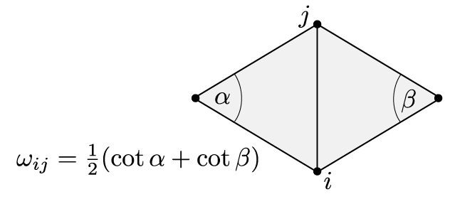
Further we have computed the Dirichlet energy of an affine function \(\hat f\) on a single triangle: If \(T_\sigma \subset \mathbb R^2\) denotes the triangle corresponding to \(\sigma=\{i,j,k\}\in F\) and \(\alpha_{jk}^i\) denotes the interior angle in \(T_\sigma\) at the vertex \(i\), then\[ \int_{T_\sigma} \bigl|\mathrm{grad}\, \hat f\bigr|^2 = \tfrac{1}{2}\bigl(\cot \alpha_{jk}^i\,(f_j – f_k)^2 +\cot \alpha_{ki}^j\,(f_k – f_i)^2 +\cot \alpha_{ij}^k\, (f_i – f_j)^2\bigr).\]The Dirichlet energy of a discrete function \(f\in \mathbb R^V\) is then defined as the Dirichlet energy of the corresponding piecewise affine function \(\hat f\):\begin{align}2\,E_D(f) & = \sum_{\sigma \in \Sigma} \int_{T_\sigma} \bigl|\mathrm{grad}\, \hat f\bigr|^2 =\sum_{\{i,j,k\} \in F} \tfrac{1}{2}\bigl(\cot \alpha_{jk}^i (f_j – f_k)^2 +\cot \alpha_{ki}^j (f_k – f_i)^2 +\cot \alpha_{ij}^k (f_i – f_j)^2\bigr)\\&=\sum_{\{i,j\} \in E} \sum_{\{i,j,k\}\in F}\tfrac{1}{2}\cot \alpha_k^{ij} (f_i – f_j)^2.\end{align}As a quadratic form the Dirichlet energy has a corresponding symmetric bilinear form: Let\[\omega_{ij} = \tfrac{1}{2}\sum_{\{i,j,k\}\in F}\cot\alpha_{ij}^k\] and define \(\mathbf L\) by \[\mathbf L_{ij} = \cases{-\sum_{{i,k}\in E}\omega_{ik},& if \(i=j\),\\\omega_{ij},& if \(\{i,j\}\in E\)\\ 0, & else,}\]then\[E_D(f) = -\tfrac{1}{2}\,f^T \mathbf L \, f.\]Note, that on a surface each edge is contained in exactly one or two triangles. Thus the weights \(\omega_{ij}\) are sums of only one or two cotangents as illustrated in the picture below for the case of an inner edge.

Now let \(\mathring V\) denote the set of interior vertices and set \(V_{bd}: = V\setminus \mathring V\). To each \(g\colon V_{bd} \to \mathbb R\) we define an affine space\[W_g := \bigl\{f\in \mathbb R^V \mid \left.f\right|_{V_{bd}}= g\bigr\}.\]Given \(g\) we are looking for a critical points of the restriction \(E_D\colon W_g \to \mathbb R\).  Therefore we compute the derivative of \(E_D\): Let \(f\in W_g\) and let \(f_t\) be a curve in \(W_g\) through \(f\) with \(X = \left.\tfrac{d}{dt}\right|_{t=0}\,f_t\). Then we get\[d_f E_D\,(X) =\left.\tfrac{d}{dt}\right|_{t=0} E_D(f_t) = -\tfrac{1}{2}\left.\tfrac{d}{dt}\right|_{t=0}\, (f_t^T \mathbf L\, f_t) =-\tfrac{1}{2}f^T \mathbf L\, X -\tfrac{1}{2}X^T \mathbf L\, f= -X^T\mathbf L\,f.\]Since \(f_t \in W_g\)  for all \(t\) we obtain that \(X\in W_0\), i.e. \(\left.X\right|_{V_{bd}} = 0\). Conversely each \(X\in W_0\) yields a curve in \(W_g\) through \(f\). Thus \(f\) is a critical point of \(E_D\) if and only if the entries of \(\mathbf L\,f\) corresponding to interior vertices vanish: For each vertex \(i\in \mathring V\) we have \[\sum_{\{i,j\}\in E} \omega_{ij}f_i-\sum_{\{i,j\}\in E} \omega_{ij}f_j =  \sum_{\{i,j\}\in E} \omega_{ij}(f_i- f_j) = 0.\]Since \(E_D\) is convex there is always a global minimum and thus there is always a solution. As in the smooth case the minimizer is unique.

To summarize: Given any function \(g\colon V_{bd}\to \mathbb R\), the unique minimizer \(f\in W_g\) of the Dirichlet energy is the solution of the following linear system\[\cases{\sum_{\{i,j\}\in E} \omega_{ij}(f_i- f_j) = 0, & for each \(i\in \mathring V\),\\f_i = g_i, & for each \(i\in V_{bd}\).}\]

Now we want to build up a network that computes the minimizer for given a function given on the boundary of a surface in \(\mathbb R^2\).

First we need to specify a surface in \(\mathbb R^2\) and a function \(g\) on its boundary. One possible way to do this is to use a space curve: First we draw with a curve node a space curve and probably resample it. Then we use the say y-component as the function \(g\) on the boundary and project it to a polygon in the plane xz-plane and remesh it. Here the network

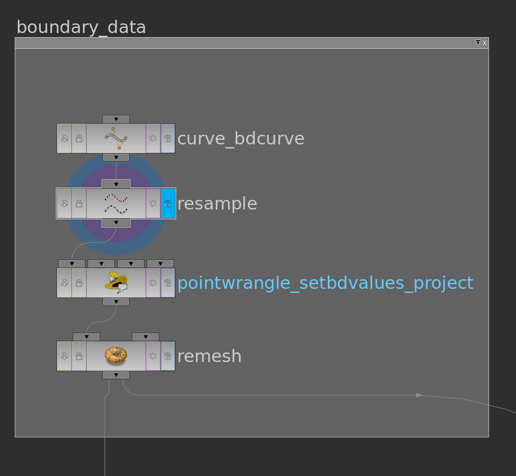
The pointwrangle node contains the following 3 lines of code:

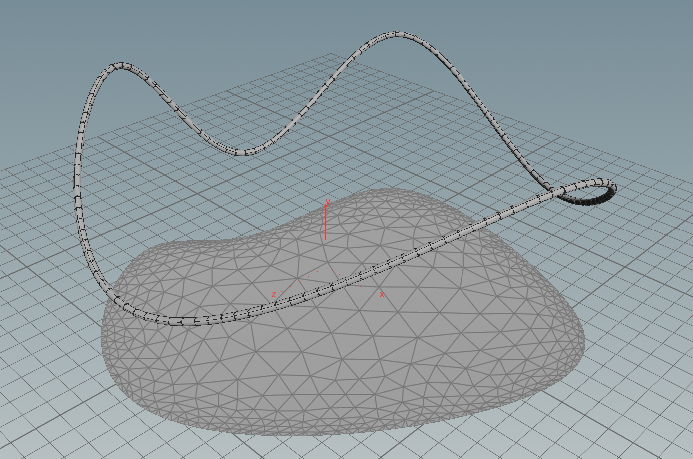
Then we have a triangulated surface in the plane and a graph over its boundary (the curve we started with).

Now we want to build up the matrix \(\mathbf A\) of the linear system. To solve the system we will use scipy. Though, for performance reasons, we will do as much as we can in VEX, which is much faster than python. In particular we will avoid python loops when filling the matrix.

We will use a compressed sparse row matrix (scipy.sparse.csr_matrix). The constructor needs 3 arrays of equal length – two integer arrays (rows,colums) specifying the position of non-zero entries and a double array that specifies the non-zero entries – and two integers that specify the format of the matrix.

The non-zero entries in \(\mathbf A\)  are exactly the diagonal entries \(\mathbf A_{ii}\) and the off-diagonal entries \(\mathbf A_{ij}\) that belong to oriented edges \(ij\) of the surface.  Accessing Houdini point attributes and Houdini primitive attributes in python is fast, but unfortunately that’s not the case for the Houdini vertex attributes. Fortunately, we can store the vertex attribute in vectors sitting on primitives: For a surface the Houdini vertices of the primitives are one-to-one with its halfedges – each vertex is the start vertex of a halfedge in the boundary of the Houdini primitive.

By this observation above we can get a complete array of non-zero value indices as follows: we can store an attribute i@id = @ptnum (@ptnum itself is not accessible from python) on points and two attributes v@start and v@end (encoding row and column resp.) on Houdini primitive that contain for each edge in the primitive (starting from primhedge(geo,@primnum)) the point number of the source point (@start) and destination point (@end) of the current edge in the Houndini primitive.

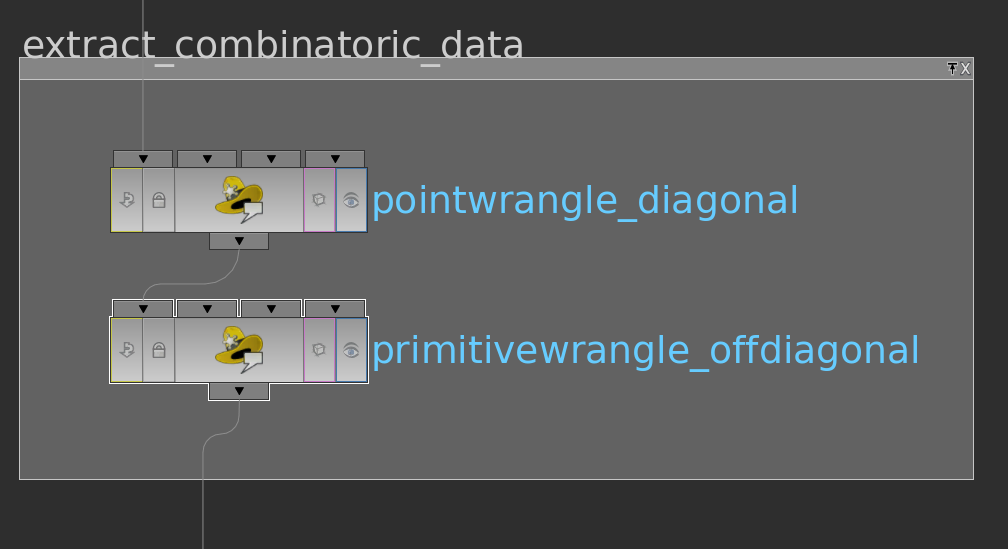
Here the VEX code of the primitivewrangle node:

The pointwrangle node just contains one line (i@id = @ptnum;).

Before we can finally start to compute the cotangent weights and write the matrix entries to attributes we still need one more information – whether a point lies on the boundary or not. This we can do e.g. as follows:

The group node has in its edge tab a toggle to detect ‘unshared edges’, i.e. edge which appear in only one triangle. With this we build a group boundary over whose points we then run with a pointwrangle node setting an attribute i@bd = 1 (the other points then have @bd = 0 per default).

Now let us start to compute the matrix entries. We will do this here in several steps.

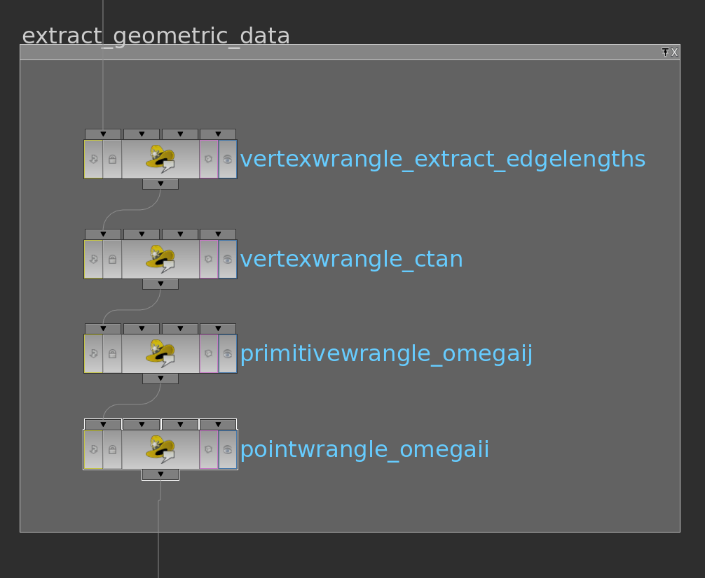
Here VEX code of the wrangle nodes in their order:

Now that we have set up the values we can build up the matrix in a python node: The attributes can read out of the Houdini geometry (geo) using methods as pointIntAttribValues(“attributename”) or primFloatAttribValues(“attributename”).  The arrays are concatenated by numpy.append and then handed over to the csr_matrix-constructor. To access the matrix in the next node we can store it as cachedUserData in the node (compare the code below).

We still need to prepare the right hand side of the system. Therefore we extend the function \(g\) defined on the boundary vertices to the interior vertices by zero (pointwrangle node) and store it as cachedUserData as well (python node).

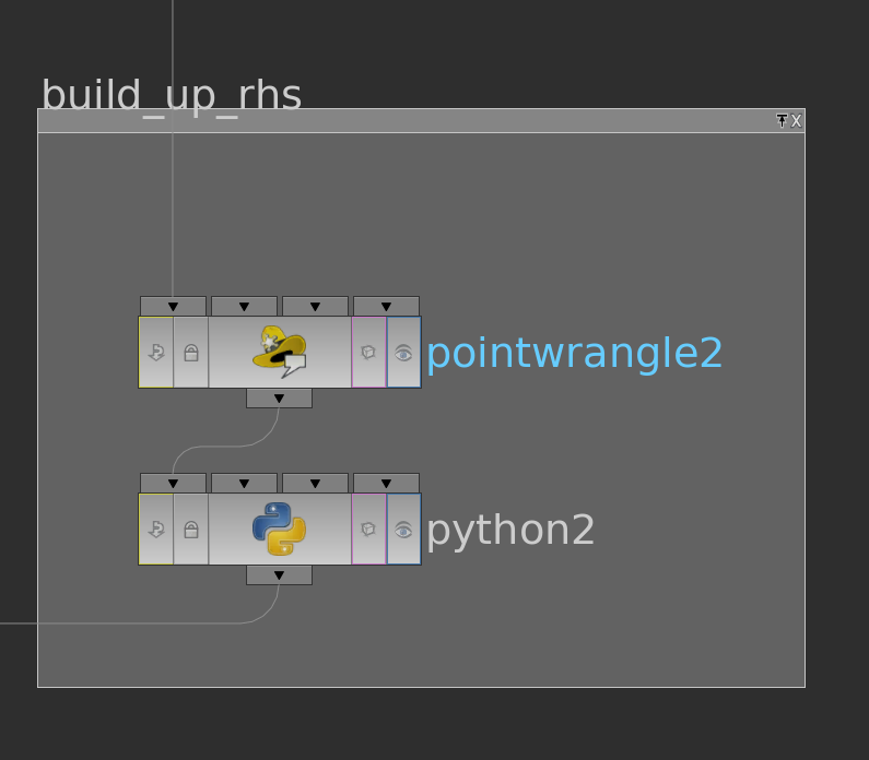
Here the corresponding code

Now we stick both python node – the one in which we stored the matrix and the one in which we stored the right hand side – into another one where we finally solve the linear system.

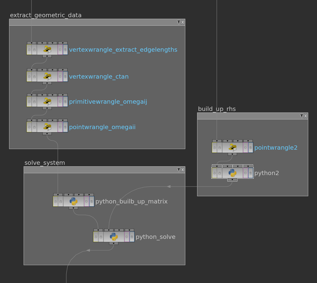
The cached user data can be accessed by its name. The easiest way to solve the system is to use scipy.sparse.linalg.spsolve. After that the solution is stored as a point attribute. Below the corresponding python code:

Though this can be speeded up when rewriting the system as an inhomogeneous symmetric system, which can then be solved by scipy.sparse.linalg.cg. Here the alternative code:

Now we are back in VEX land and we can finally draw the graph of the solution:

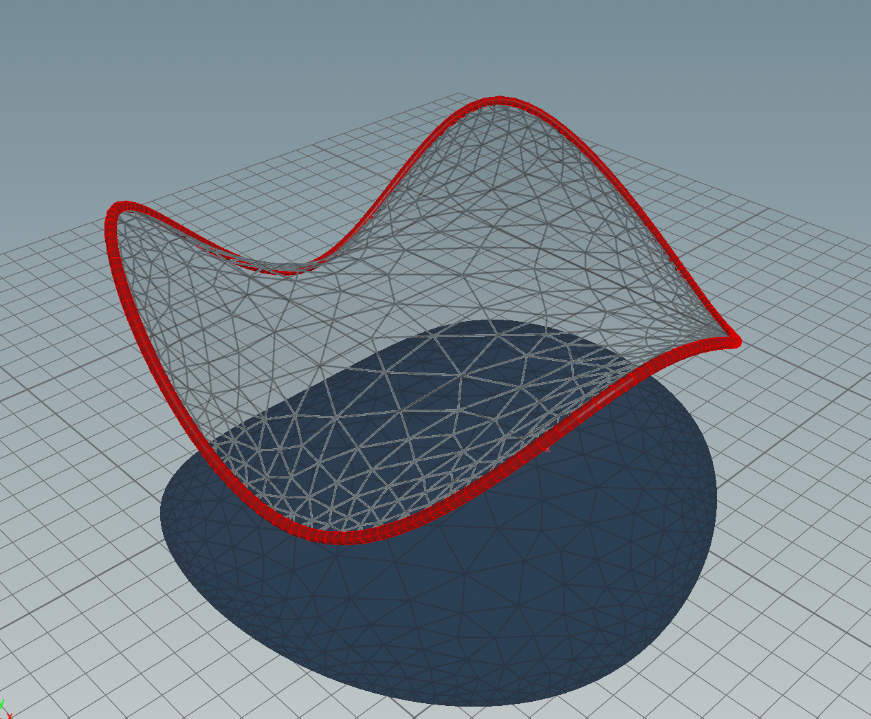
Homework (due 5/7 July). Build a network which allows to prescribe boundary values and then computes the corresponding minimizer of the Dirichlet energy.