Tutorial 9 – The Dirichlet problem

In the lecture we saw that the Dirichlet energy has a unique minimizer among all functions with prescribed boundary values. In this tutorial we want to visualize these minimizers in the discrete setting.

Let \(\mathrm M\subset \mathbb R^2\) be a triangulated surface with boundary \(\partial \mathrm M\) and let \(V\), \(E\)  and \(F\) denote the set of vertices, edges and triangles of the underlying simplicial complex \(\Sigma\). Further, let \(p_i\in \mathbb R^2\) denote the position of the vertex \(i\in V\).

To each discrete function \(f\in\mathbb R^V\) we assigned a corresponding piecewise affine function \(\hat f=\sum_{i\in V}f_i\phi_i\). Here \(\phi_i\) denotes the hat function corresponding to the vertex \(i\), i.e. \(\phi_i\) is the unique piecewise affine function such that \(\phi_i(p_j) = \delta_{ij}\).

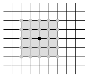
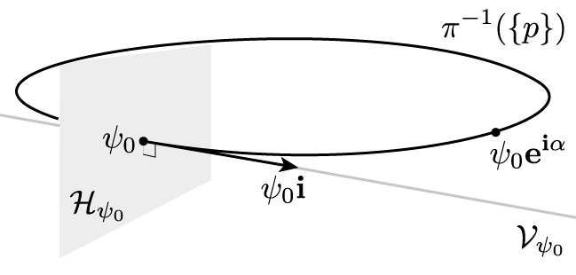
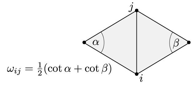
Further we have computed the Dirichlet energy of an affine function \(\hat f\) on a single triangle: If \(T_\sigma \subset \mathbb R^2\) denotes the triangle corresponding to \(\sigma=\{i,j,k\}\in F\) and \(\alpha_{jk}^i\) denotes the interior angle in \(T_\sigma\) at the vertex \(i\), then\[ \int_{T_\sigma} \bigl|\mathrm{grad}\, \hat f\bigr|^2 = \tfrac{1}{2}\bigl(\cot \alpha_{jk}^i\,(f_j – f_k)^2 +\cot \alpha_{ki}^j\,(f_k – f_i)^2 +\cot \alpha_{ij}^k\, (f_i – f_j)^2\bigr).\]The Dirichlet energy of a discrete function \(f\in \mathbb R^V\) is then defined as the Dirichlet energy of the corresponding piecewise affine function \(\hat f\):\begin{align}2\,E_D(f) & = \sum_{\sigma \in \Sigma} \int_{T_\sigma} \bigl|\mathrm{grad}\, \hat f\bigr|^2 =\sum_{\{i,j,k\} \in F} \tfrac{1}{2}\bigl(\cot \alpha_{jk}^i (f_j – f_k)^2 +\cot \alpha_{ki}^j (f_k – f_i)^2 +\cot \alpha_{ij}^k (f_i – f_j)^2\bigr)\\&=\sum_{\{i,j\} \in E} \sum_{\{i,j,k\}\in F}\tfrac{1}{2}\cot \alpha_k^{ij} (f_i – f_j)^2.\end{align}As a quadratic form the Dirichlet energy has a corresponding symmetric bilinear form: Let\[\omega_{ij} = \tfrac{1}{2}\sum_{\{i,j,k\}\in F}\cot\alpha_{ij}^k\] and define \(\mathbf L\) by \[\mathbf L_{ij} = \cases{-\sum_{{i,k}\in E}\omega_{ik},& if \(i=j\),\\\omega_{ij},& if \(\{i,j\}\in E\)\\ 0, & else,}\]then\[E_D(f) = -\tfrac{1}{2}\,f^T \mathbf L \, f.\]Note, that on a surface each edge is contained in exactly one or two triangles. Thus the weights \(\omega_{ij}\) are sums of only one or two cotangents as illustrated in the picture below for the case of an inner edge.

cotanweights

Now let \(\mathring V\) denote the set of interior vertices and set \(V_{bd}: = V\setminus \mathring V\). To each \(g\colon V_{bd} \to \mathbb R\) we define an affine space\[W_g := \bigl\{f\in \mathbb R^V \mid \left.f\right|_{V_{bd}}= g\bigr\}.\]Given \(g\) we are looking for a critical points of the restriction \(E_D\colon W_g \to \mathbb R\).  Therefore we compute the derivative of \(E_D\): Let \(f\in W_g\) and let \(f_t\) be a curve in \(W_g\) through \(f\) with \(X = \left.\tfrac{d}{dt}\right|_{t=0}\,f_t\). Then we get\[d_f E_D\,(X) =\left.\tfrac{d}{dt}\right|_{t=0} E_D(f_t) = -\tfrac{1}{2}\left.\tfrac{d}{dt}\right|_{t=0}\, (f_t^T \mathbf L\, f_t) =-\tfrac{1}{2}f^T \mathbf L\, X -\tfrac{1}{2}X^T \mathbf L\, f= -X^T\mathbf L\,f.\]Since \(f_t \in W_g\)  for all \(t\) we obtain that \(X\in W_0\), i.e. \(\left.X\right|_{V_{bd}} = 0\). Conversely each \(X\in W_0\) yields a curve in \(W_g\) through \(f\). Thus \(f\) is a critical point of \(E_D\) if and only if the entries of \(\mathbf L\,f\) corresponding to interior vertices vanish: For each vertex \(i\in \mathring V\) we have \[\sum_{\{i,j\}\in E} \omega_{ij}f_i-\sum_{\{i,j\}\in E} \omega_{ij}f_j =  \sum_{\{i,j\}\in E} \omega_{ij}(f_i- f_j) = 0.\]Since \(E_D\) is convex there is always a global minimum and thus there is always a solution. As in the smooth case the minimizer is unique.

To summarize: Given any function \(g\colon V_{bd}\to \mathbb R\), the unique minimizer \(f\in W_g\) of the Dirichlet energy is the solution of the following linear system\[\cases{\sum_{\{i,j\}\in E} \omega_{ij}(f_i- f_j) = 0, & for each \(i\in \mathring V\),\\f_i = g_i, & for each \(i\in V_{bd}\).}\]

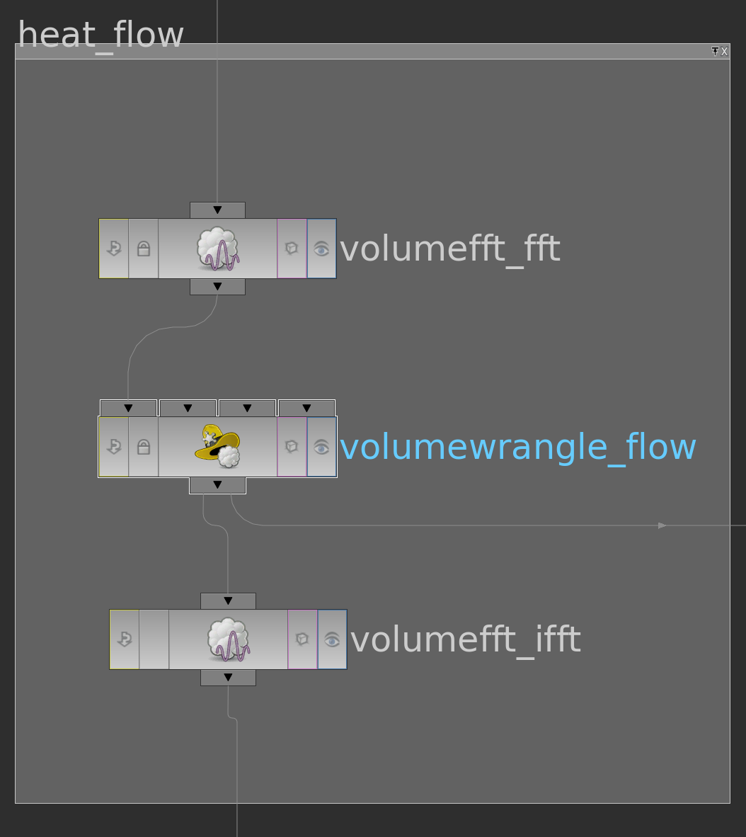
Now we want to build up a network that computes the minimizer for given a function given on the boundary of a surface in \(\mathbb R^2\).

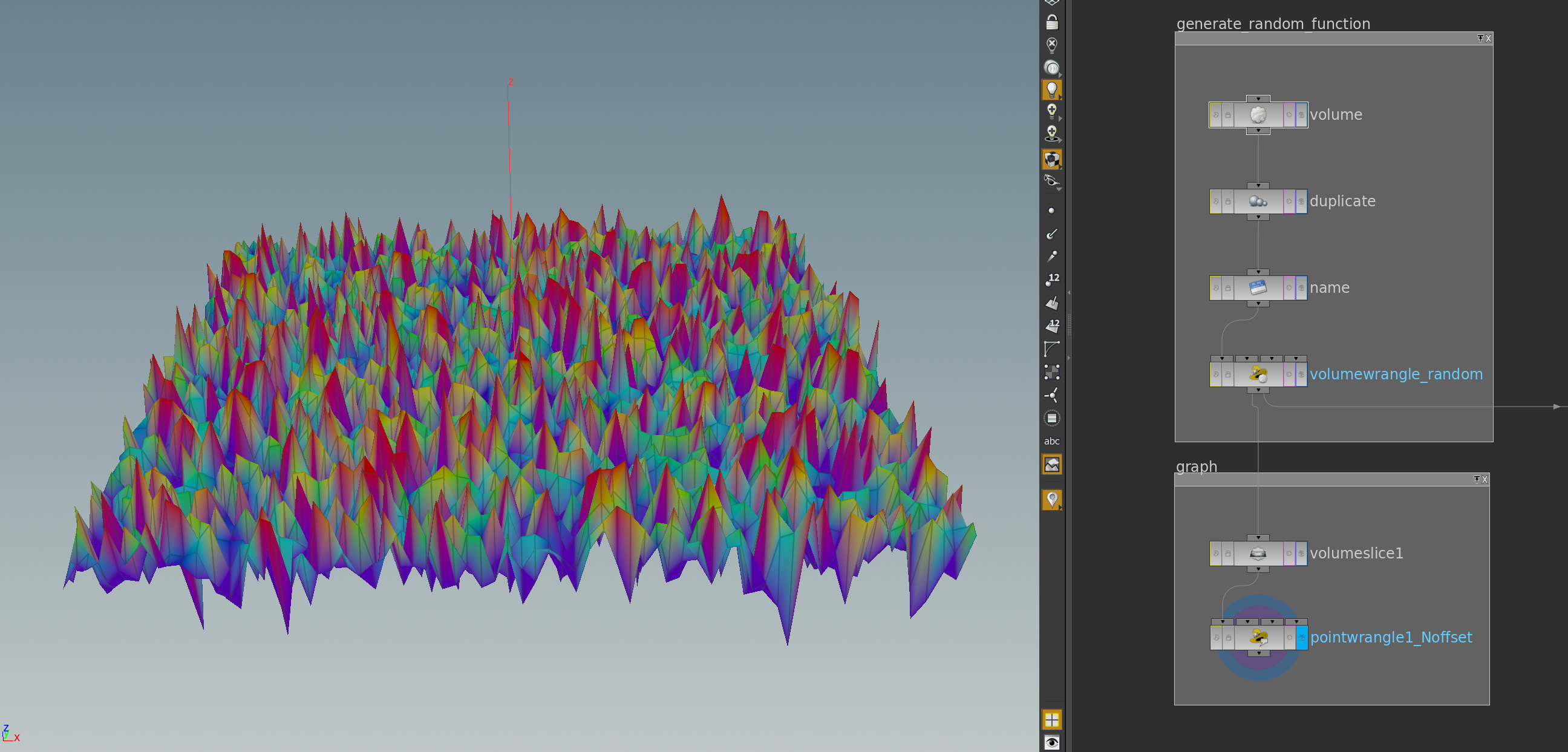
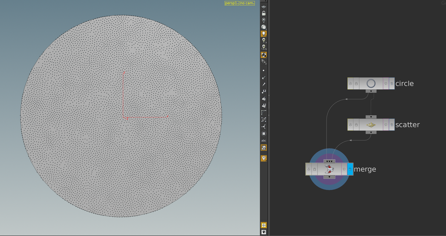
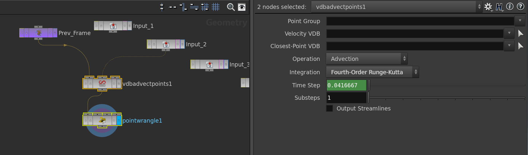
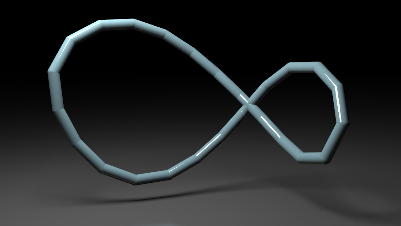
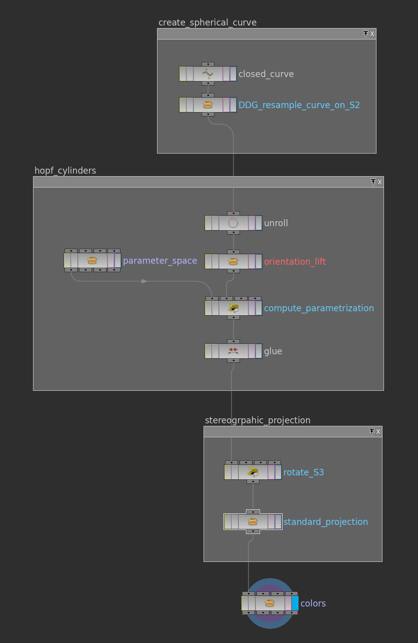
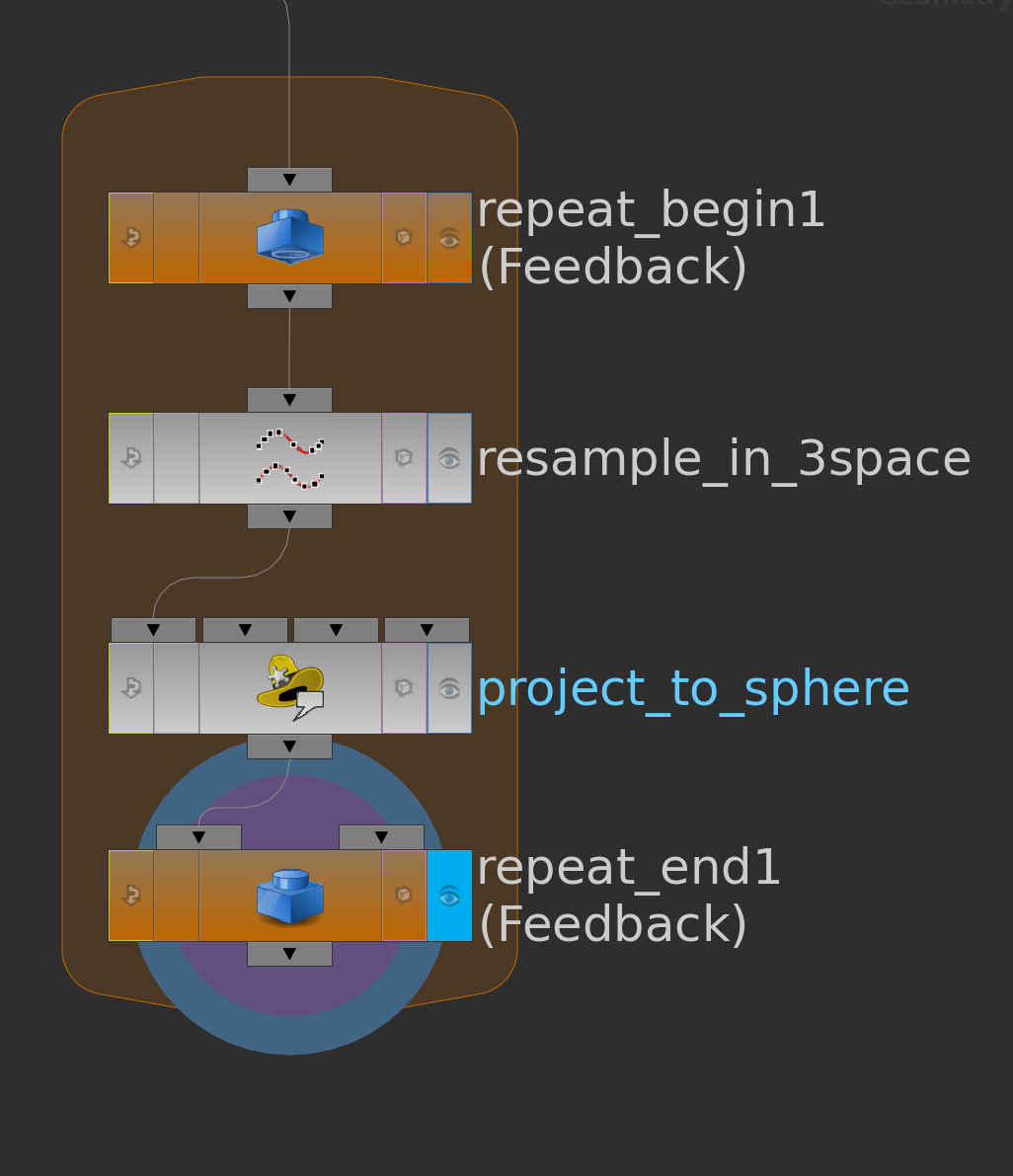
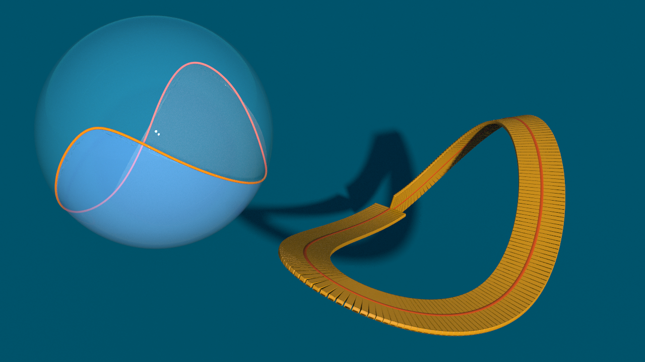
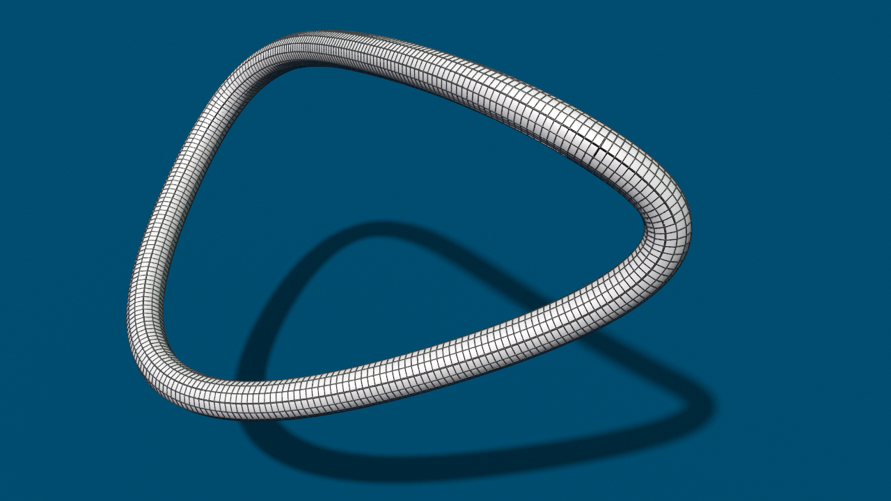
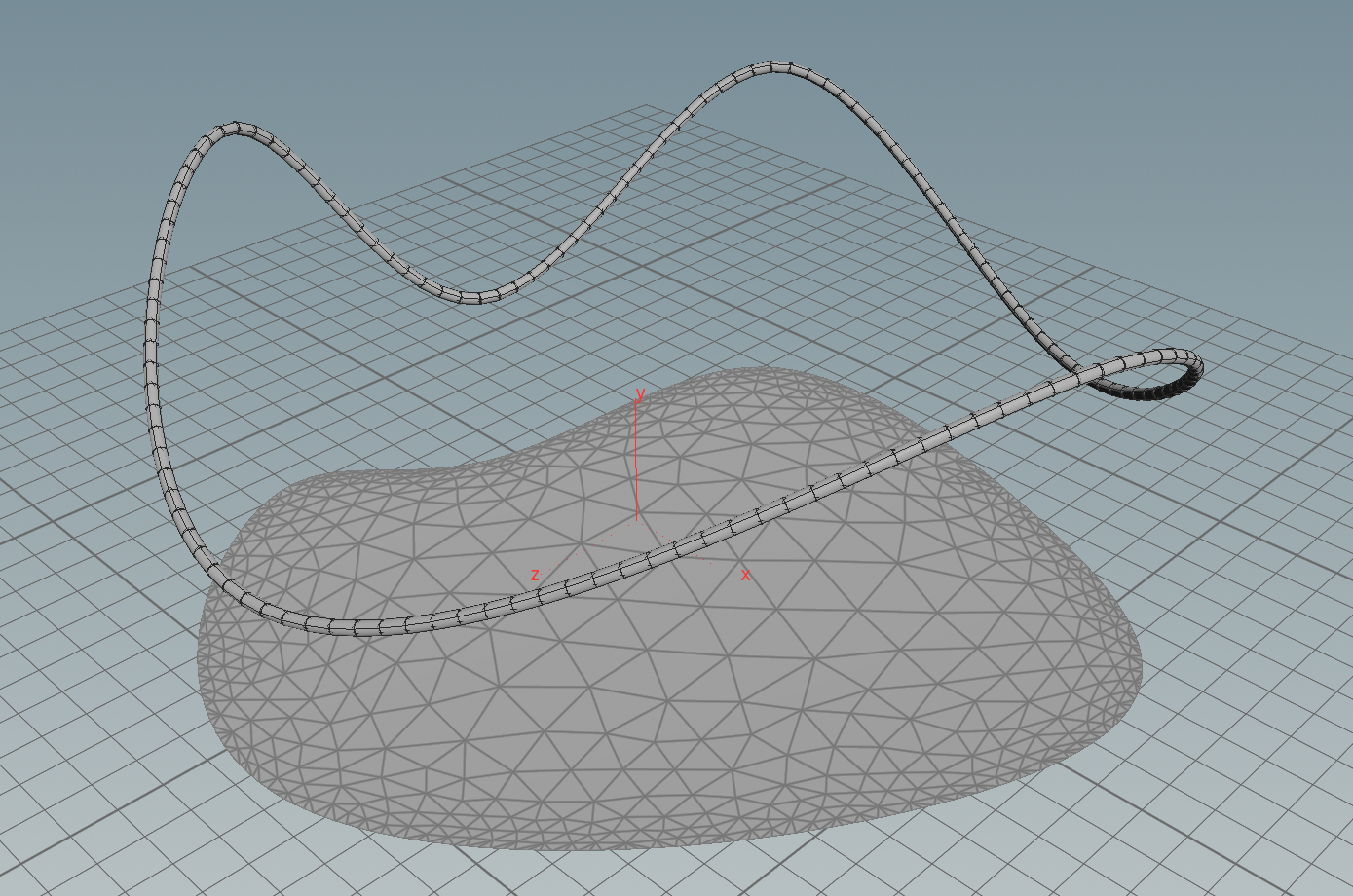
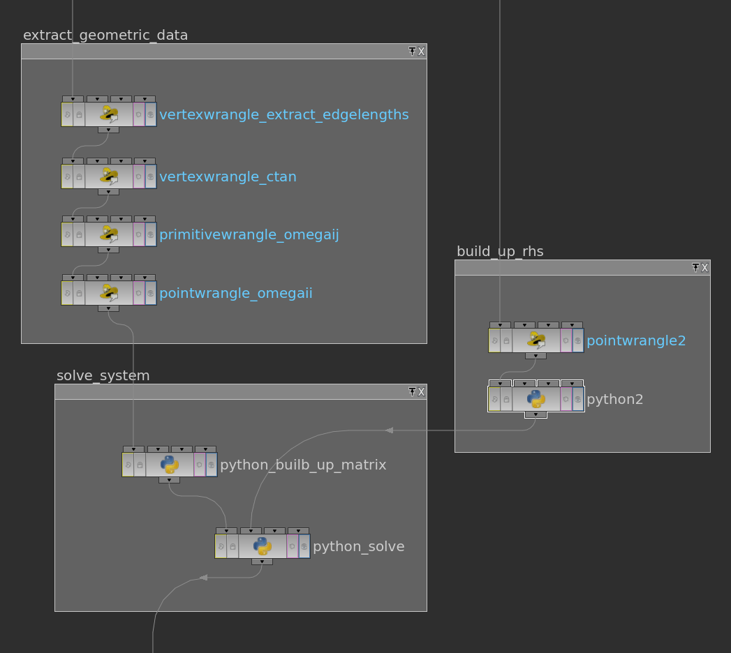
First we need to specify a surface in \(\mathbb R^2\) and a function \(g\) on its boundary. One possible way to do this is to use a space curve: First we draw with a curve node a space curve and probably resample it. Then we use the say y-component as the function \(g\) on the boundary and project it to a polygon in the plane xz-plane and remesh it. Here the network

boundary_datanetwork

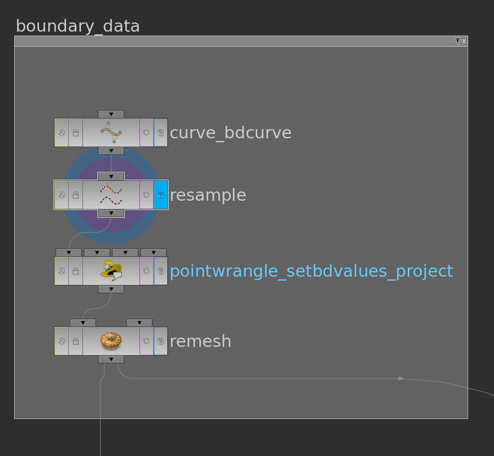
The pointwrangle node contains the following 3 lines of code:

Then we have a triangulated surface in the plane and a graph over its boundary (the curve we started with).

specifyingboundarydata

Now we want to build up the matrix \(\mathbf A\) of the linear system. To solve the system we will use scipy. Though, for performance reasons, we will do as much as we can in VEX, which is much faster than python. In particular we will avoid python loops when filling the matrix.

We will use a compressed sparse row matrix (scipy.sparse.csr_matrix). The constructor needs 3 arrays of equal length – two integer arrays (rows,colums) specifying the position of non-zero entries and a double array that specifies the non-zero entries – and two integers that specify the format of the matrix.

The non-zero entries in \(\mathbf A\)  are exactly the diagonal entries \(\mathbf A_{ii}\) and the off-diagonal entries \(\mathbf A_{ij}\) that belong to oriented edges \(ij\) of the surface.  Accessing Houdini point attributes and Houdini primitive attributes in python is fast, but unfortunately that’s not the case for the Houdini vertex attributes. Fortunately, we can store the vertex attribute in vectors sitting on primitives: For a surface the Houdini vertices of the primitives are one-to-one with its halfedges – each vertex is the start vertex of a halfedge in the boundary of the Houdini primitive.

By this observation above we can get a complete array of non-zero value indices as follows: we can store an attribute i@id = @ptnum (@ptnum itself is not accessible from python) on points and two attributes v@start and v@end (encoding row and column resp.) on Houdini primitive that contain for each edge in the primitive (starting from primhedge(geo,@primnum)) the point number of the source point (@start) and destination point (@end) of the current edge in the Houndini primitive.

extractcombinatorics

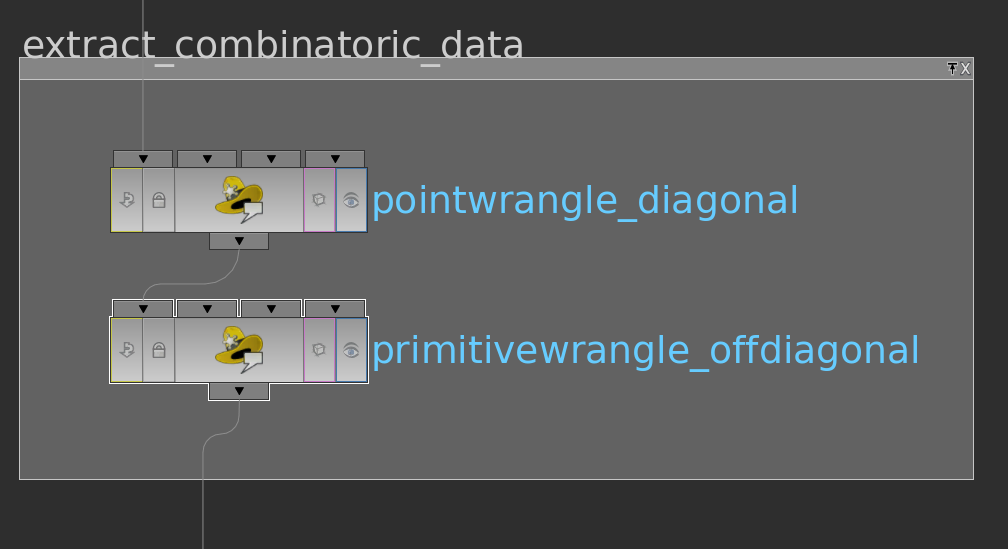
Here the VEX code of the primitivewrangle node:

The pointwrangle node just contains one line (i@id = @ptnum;).

Before we can finally start to compute the cotangent weights and write the matrix entries to attributes we still need one more information – whether a point lies on the boundary or not. This we can do e.g. as follows:

boundarypoints

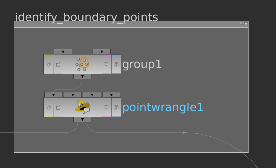
The group node has in its edge tab a toggle to detect ‘unshared edges’, i.e. edge which appear in only one triangle. With this we build a group boundary over whose points we then run with a pointwrangle node setting an attribute i@bd = 1 (the other points then have @bd = 0 per default).

Now let us start to compute the matrix entries. We will do this here in several steps.

matrixentries

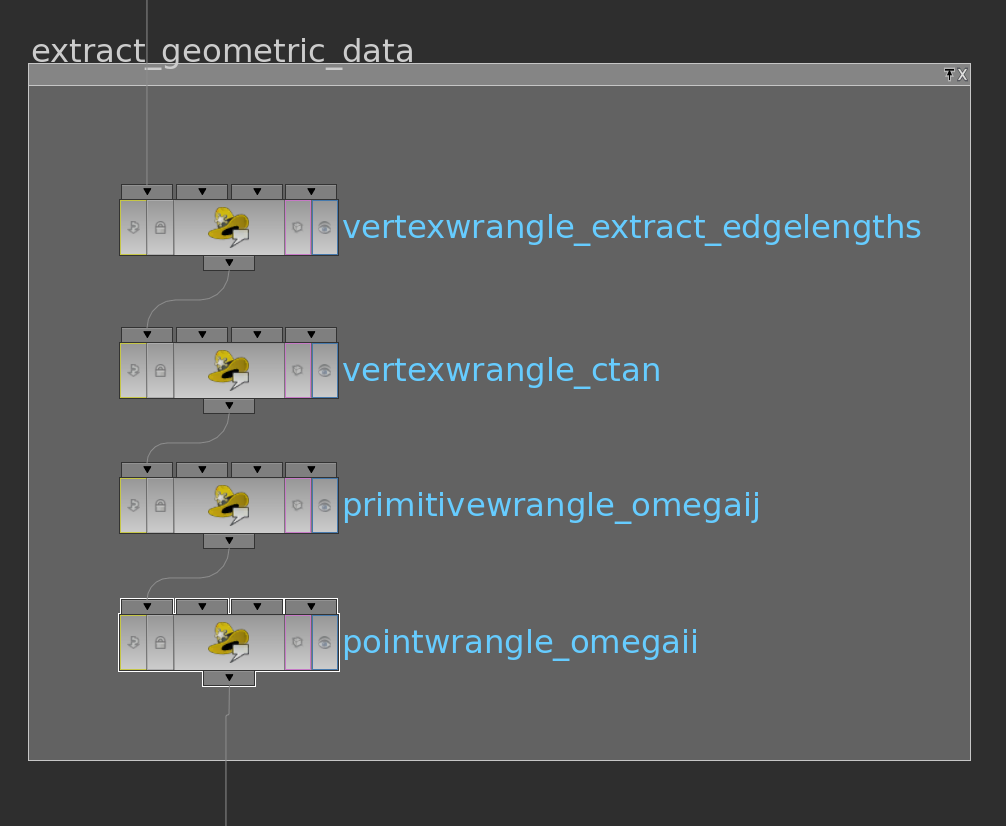
Here VEX code of the wrangle nodes in their order:

Now that we have set up the values we can build up the matrix in a python node: The attributes can read out of the Houdini geometry (geo) using methods as pointIntAttribValues(“attributename”) or primFloatAttribValues(“attributename”).  The arrays are concatenated by numpy.append and then handed over to the csr_matrix-constructor. To access the matrix in the next node we can store it as cachedUserData in the node (compare the code below).

We still need to prepare the right hand side of the system. Therefore we extend the function \(g\) defined on the boundary vertices to the interior vertices by zero (pointwrangle node) and store it as cachedUserData as well (python node).

rhs

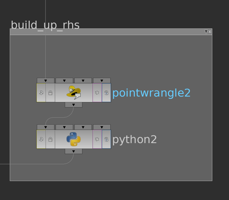
Here the corresponding code

Now we stick both python node – the one in which we stored the matrix and the one in which we stored the right hand side – into another one where we finally solve the linear system.

solvesystem

The cached user data can be accessed by its name. The easiest way to solve the system is to use scipy.sparse.linalg.spsolve. After that the solution is stored as a point attribute. Below the corresponding python code:

Though this can be speeded up when rewriting the system as an inhomogeneous symmetric system, which can then be solved by scipy.sparse.linalg.cg. Here the alternative code:

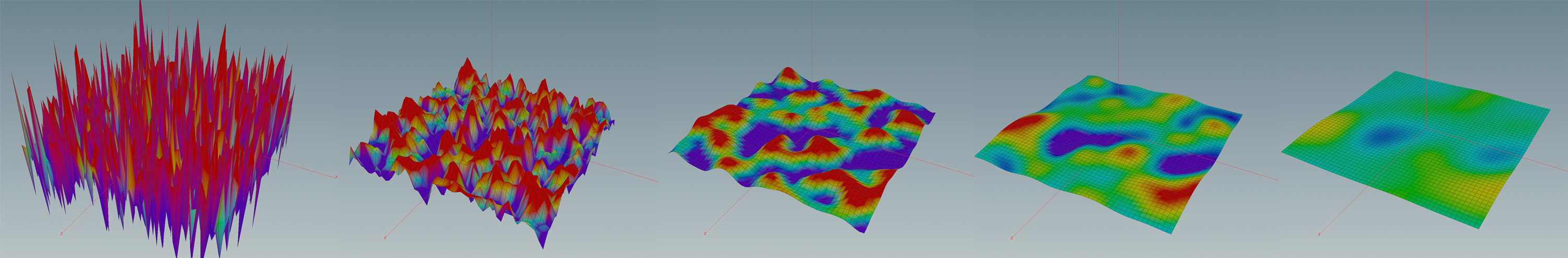
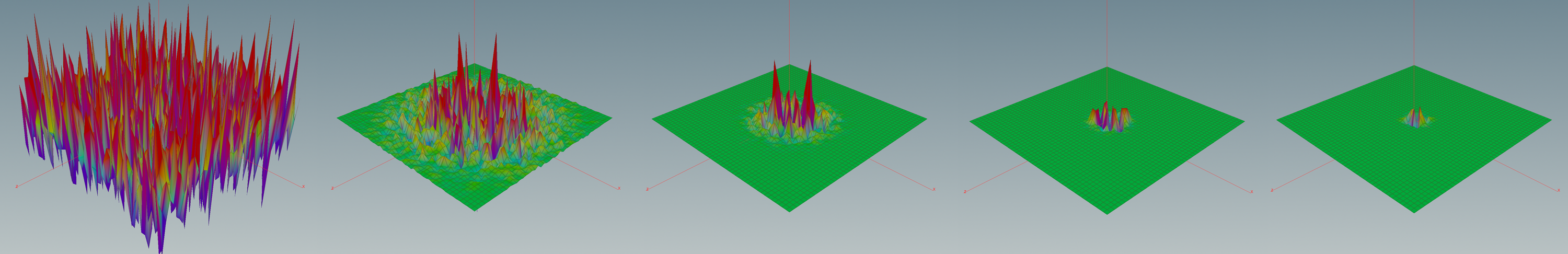
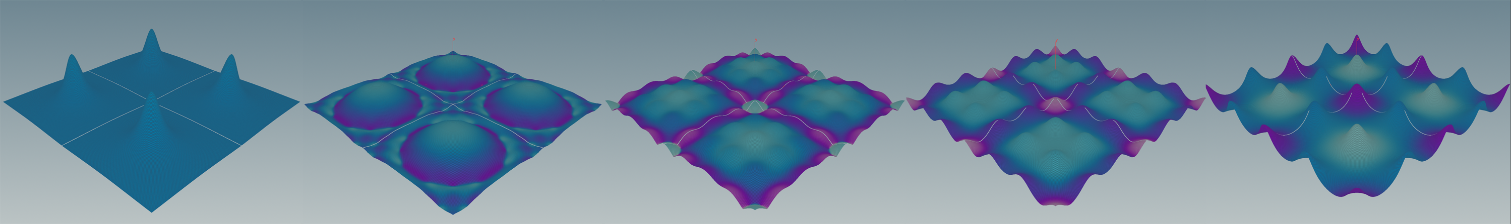
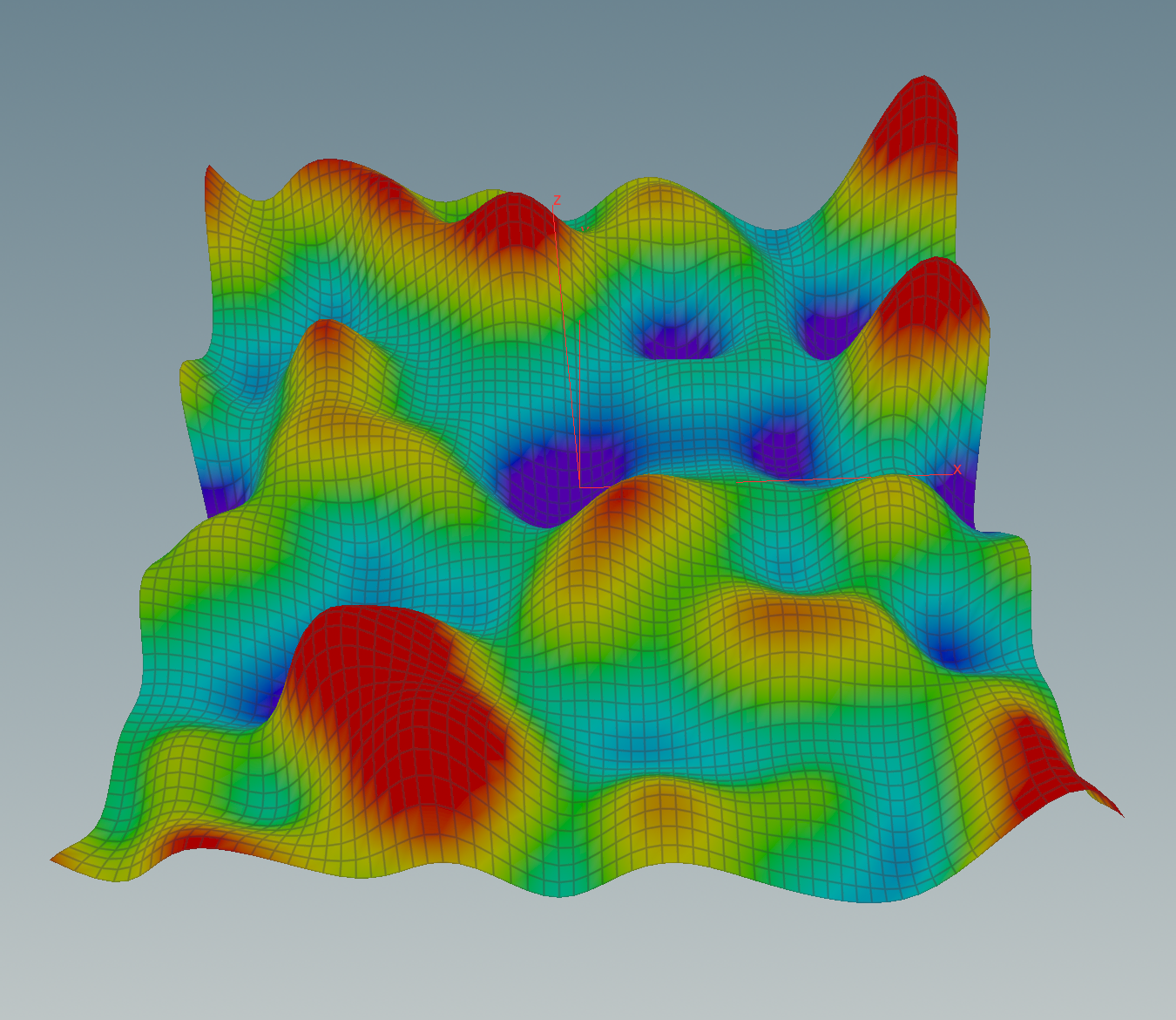
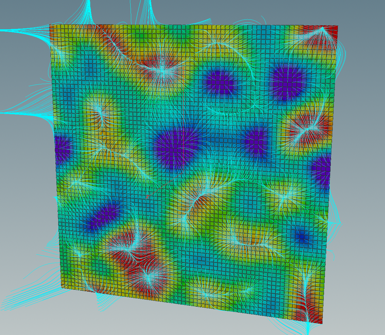
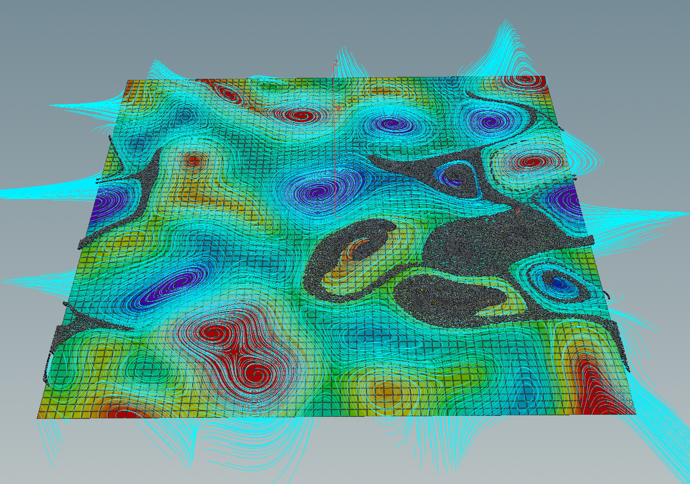
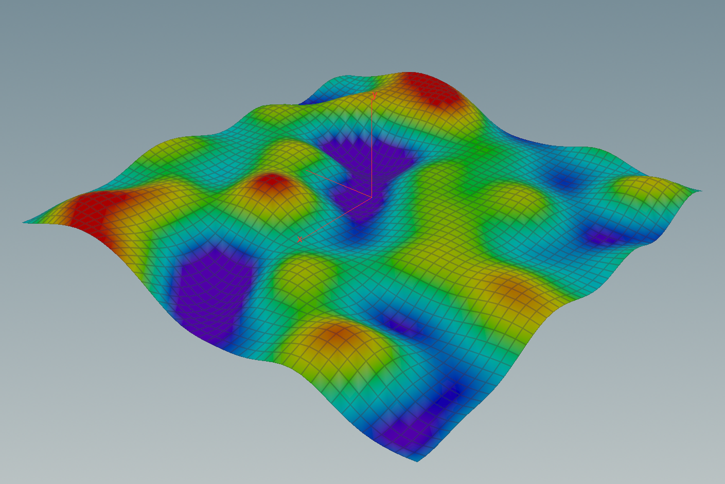
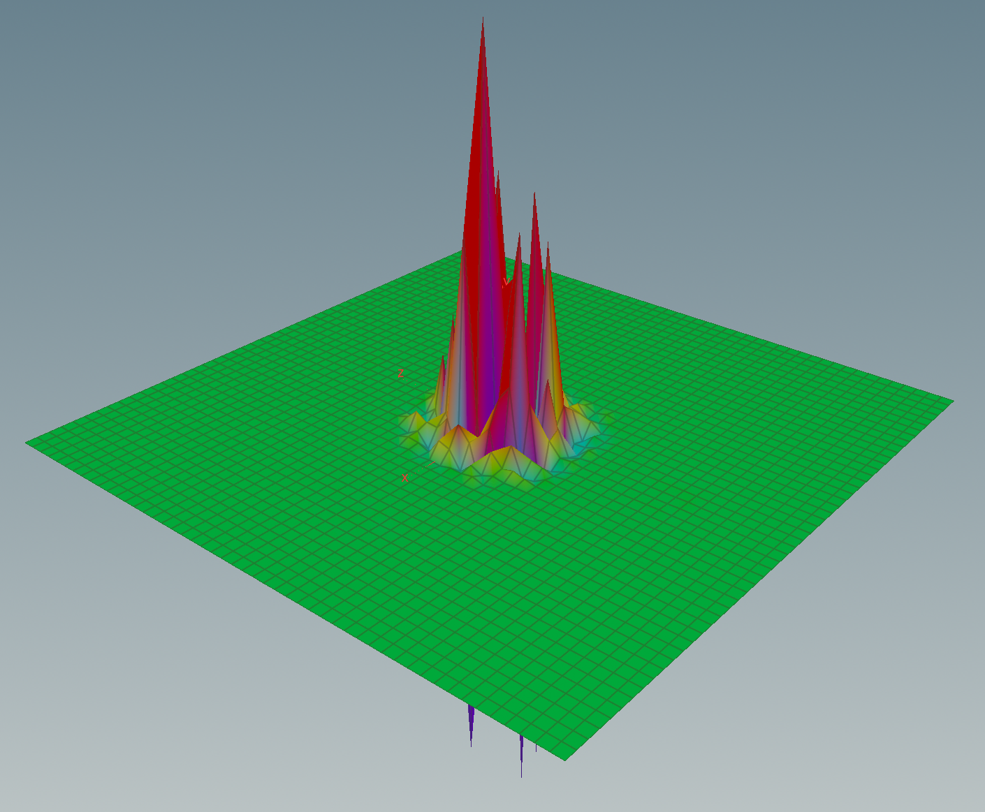
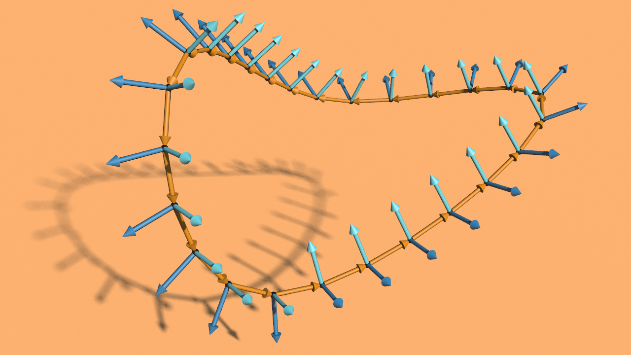
Now we are back in VEX land and we can finally draw the graph of the solution:

harmonicgraph

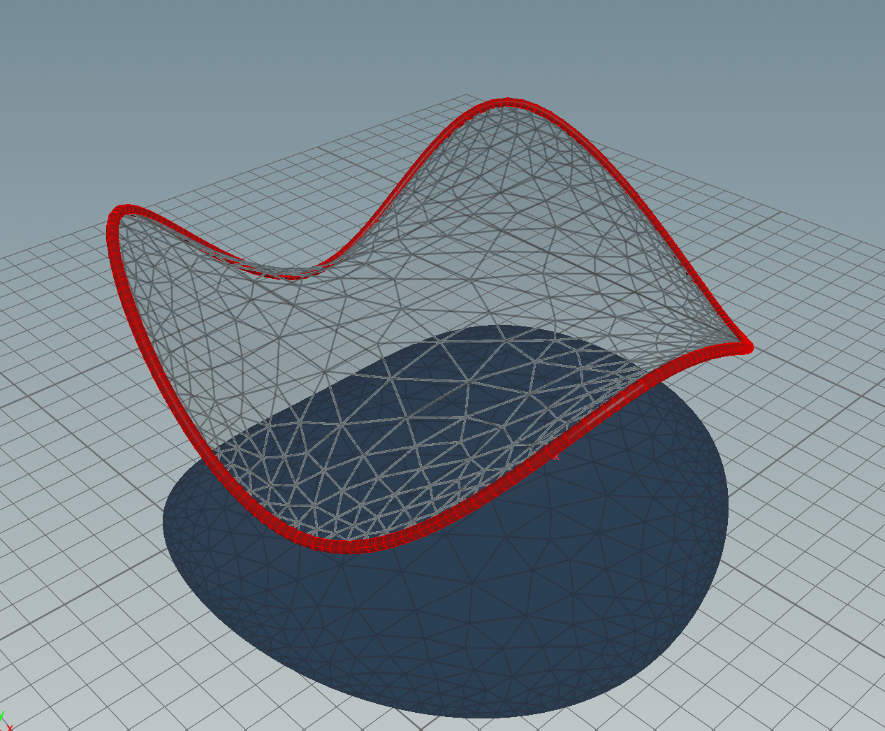
Homework (due 5/7 July). Build a network which allows to prescribe boundary values and then computes the corresponding minimizer of the Dirichlet energy.

Posted in Tutorial | Comments Off on Tutorial 9 – The Dirichlet problem

Tutorial 8 – Flows on functions

Last time we looked at the gradient flows of functions defined on the torus \(\mathrm T^n\). This time we will look at flows on the space of Fourier polynomials \(\mathcal F_N\).

Let us first restrict ourselves to the real-valued Fourier polynomials \(\mathcal F_N^{\mathbb R} \subset \mathcal F_N\).  The space \(\mathcal F_N^{\mathbb R}\) is a finite-dimensional Hilbert space and we can define the derivative of functionals and their gradient as usual: Let \(H\colon \mathcal F_N^{\mathbb R} \to \mathbb R\) be a smooth functional. Then, for \(f\in \mathcal F_N^{\mathbb R}\) and \(X\in \mathcal F_N^{\mathbb R}\),\[d_{f}H (X) =: \langle\!\langle \mathrm{grad}_f H , X\rangle\!\rangle.\]One of the most prominent functionals is the so called Dirichlet energy \(E_D\), which is defined as half the \(L^2\)-norm of the gradient: For \(f\in \mathcal F_N^{\mathbb R}\), \[E_D(f) : = \tfrac{1}{2}\int_{\mathrm T^n} |\mathrm{grad}\, f|^2 =\tfrac{1}{2}\Vert \mathrm{grad}\, f \Vert^2.\]As such the Dirichlet energy measures the ‘smoothness’ of the function. Certainly, \(E_D(f)\geq 0\) and, since \(\mathrm T^n\) is connected, we have\[f= const \Longleftrightarrow \mathrm{grad}\, f = 0 \Longleftrightarrow E_D(f) = 0.\]The Dirichlet energy is closely related to the Laplace operator \(\Delta := \mathrm{div}\circ\mathrm{grad}\).

Theorem 1. For smooth \(f,g\colon \mathrm{T^n} \to \mathbb R\), we have \(\langle\!\langle \mathrm{grad}\, f,\mathrm{grad}\, g\rangle\!\rangle = -\langle\!\langle f,\Delta g\rangle\!\rangle\).

Proof. This following from the divergence theorem and the periodicity of \(f\mathrm{grad}\, g\): From vector calculus we know that for a smooth function \(f\) and a smooth vector field \(X\) we have the following ‘product’ rule\[\mathrm{div}(fX) = \langle \mathrm{grad}\, f,X\rangle + f\mathrm{div}(X).\]Hence, with \(X= \mathrm{grad}\,g\), the divergence theorem yields\begin{align}\langle\!\langle \mathrm{grad}\, f,\mathrm{grad}\, g\rangle\!\rangle &= \int_{\mathrm{T}^n} \langle \mathrm{grad}\, f,\mathrm{grad}\, g\rangle\\ &= \int_{\mathrm{T}^n} \mathrm{div}(f\mathrm{grad}\, g) – f\mathrm{div}(\mathrm{grad}\, g) \\&= \int_{\partial \mathrm{T}^n} \langle f\mathrm{grad}\, g,N\rangle – \int_{\mathrm{T}^n}f\mathrm{div}(\mathrm{grad}\, g) \\ &= -\int_{\mathrm{T}^n} f\mathrm{div}(\mathrm{grad}\, g) \\ &= -\langle\!\langle f, \Delta g\rangle\!\rangle.\end{align}Here \(\int_{\partial \mathrm{T}^n} \langle f\mathrm{grad}\,g, N \rangle = 0\) because of the periodicity of \(f\mathrm{grad}\,g\) – the boundary integrals of opposite sides of the fundamental domain (cube) cancel. \(\square\)

Corollary 1. The Laplace operator on the torus is self-adjoint: \(\Delta^\ast = \Delta\).

Corollary 2. The gradient of the Dirichlet energy is given by \(\mathrm{grad}_f E_D= -\Delta f\).

The gradient flow of the Dirichlet energy is well-known in Physics. It is the heat equation, \[\dot f = -\mathrm{grad}_f E_D= \Delta f,\]which describes how temperature distributes in the torus.

In coordinates the Laplace operator takes the usual form: If \(x_j\) denote the canonical coordinates on \(\mathbb R^n\), then\[\Delta f = \mathrm{div}(\mathrm{grad}\,f) = \sum_{i=j}^n \tfrac{\partial^2}{\partial x_j^2}f.\]Note, if \(\mathbf e_k\) is a vector of the Fourier basis, then \(\tfrac{\partial}{\partial x_j}\mathbf{e}_k = ik_j\,\mathbf{e}_k\) and hence \(\Delta \mathbf e_k = -|k|^2\mathbf e_k\). In particular the Laplacian restricts to a linear \(\mathcal F_N^{\mathbb R} \to\mathcal F_N^{\mathbb R}\) and is in fact diagonal with respect to the Fourier basis. The flow is easily computed: If \(f\in \sum_{k}c_k\mathbf e_k \mathcal F_N^{\mathbb R}\), \[\sum_k \dot c_k\mathbf e_k = \dot f = \Delta f = -\sum_k |k|^2c_k \mathbf e_k.\]Hence the coefficients solve \(\dot c_k = -|k|^2c_k\) and the flow is explicitly given as follows:\[c_k^t = e^{-|k|^2t}c_k^0.\]The heat flow is easily implemented in a small network involving two VolumeFFT nodes (for FFT and iFFT) and a VolumeWrangle node:

fft_flow_network

The VEX code is really simple:

Here the resulting flow starting with a random function:

heatflow_severaltimes

That the flow take us to the ‘constant part’ of the initial value \(f\) is obvious from the explicit form. The only coefficient that survives is \(c_0\) – this coefficient stays fixed under the flow. Moreover, \(c_0 = \langle\!\langle f, \mathbf e_0\rangle\!\rangle = \int_{\mathrm T^n} f/\int_{\mathrm{T}^n} 1 = \int_{\mathrm T^n} f/ \mathrm{vol}(\mathrm{T}^n)\). Thus, at each point \(p\in \mathrm{T}^n\), \(f_t(p)\) tends to the mean-value of \(f\) – as expected from the physical point of view. We can also look at the flow in Fourier domain (below we only show the real part). Here we see that all coefficients up to the one in the middle (corresponding to \(k=0\)) die off – the faster the higher the frequency, i.e. the further away from the center.

heatflow_fourierdomain

Here as we started with a random function the mean-value is expected close to zero – so seemingly nothing is left.

Now let us look at the space of complex-valued functions \(\mathcal F_N\). We can treat \(\mathcal F_N\) as a real vector space (of twice the dimension of \(\mathcal F^{\mathbb R}_N\)). The real part \(\langle\!\langle.,.\rangle\!\rangle = \mathrm{Re}\langle\!\langle.,.\rangle\!\rangle_{\mathbb C}\) of the hermitian inner product\[\langle\!\langle \psi,\phi\rangle\!\rangle_{\mathbb C} = \int_{\mathrm T^n}\overline{\psi}\phi, \quad \psi,\phi\in\mathcal F_N,\]turns \(\mathcal F_N\) into a Euclidean vector space and we can define the gradient of a smooth functional \(H\colon \mathcal F_N \to \mathbb R\) as before.

Note that if \(\psi = f+ig\) and \(\phi = u+iv\), then \(f,g,u,v \in \mathcal F_N^{\mathbb R}\) and we have\[\langle\!\langle \psi,\phi\rangle\!\rangle = \mathrm{Re}\int_{\mathrm T^n}\overline{\psi}\phi = \int_{\mathrm T^n}\mathrm{Re}\bigl((f-ig)(u+iv)\bigr) = \int_{\mathrm T^n} (fu+gv) = \langle\!\langle f,u\rangle\!\rangle + \langle\!\langle g, v\rangle\!\rangle.\]Further \(\Delta \phi = \Delta u + i\Delta v\) and thus \(\langle\!\langle \psi,\Delta \phi\rangle\!\rangle = \langle\!\langle f,\Delta u\rangle\!\rangle + \langle\!\langle g, \Delta v\rangle\!\rangle\). Hence we also have in the complex-valued case that\[\mathrm{grad}_\psi E_D = -\Delta \psi.\]Moreover, the imaginary part of the hermitian inner product yields a non-degenerate skew-symmetric bilinear form \(\sigma\) – a symplectic form,\[\sigma(X,Y) = \mathrm{Im}\langle\!\langle X, Y\rangle\!\rangle,\]which we can use to define a symplectic gradient. Certainly, the symplectic forms \(\sigma\) and the real inner product \(\langle\!\langle .,.\rangle\!\rangle\) satisfy the following relation:\[\sigma(X,Y) = \langle\!\langle i X, Y\rangle\!\rangle.\]Thus, for any smooth functional \(H\colon \mathcal F_N \to \mathbb R\), we have\[\mathrm{sgrad}_{\psi} H = -i\,\mathrm{grad}_\psi H .\]One easily shows the following theorem.

Theorem 2. If \(\gamma\) is an integral curve of \(\mathrm{sgrad}\,H\), then \(H\circ\gamma = const\).

Proof. We just have to differentiate \(H\circ \gamma\):\[\frac{d}{dt} (H\circ\gamma) = d_\gamma H(\frac{d}{dt}\gamma) = d_\gamma H(\mathrm{sgrad}_\gamma H) = -\langle\!\langle \mathrm{grad}_{\gamma}H,i\mathrm{grad}_\gamma H\rangle\!\rangle = 0.\]Thus \(H\circ\gamma\) is constant. \(\square\)

The flow of \(\mathrm{sgrad}\,E_D\) preserves the Dirichlet energy and is well-known in Physics: Actually, \(\dot\psi = \mathrm{sgrad}_\psi E_D\) is the famous (linear) Schrödinger equation\[i\dot\psi = \Delta \psi,\]which plays an important role in quantum mechanics. Again we can easily solve this equation in Fourier domain: The flow on the coefficients is given by\[c_k^t = e^{i|k|^2t}c_k^0.\]The network looks as for the heat equation – only the VEX code changes slightly:

Since we are dealing with complex-valued functions now, we need to come up with a way to visualize them. One common way to do this is to visualize the magnitude of the complex number as graph and the phase by colors. Therefore one has to come up with a suitable (periodic) color map. To set the colors we can directly set the @Cg-attribute using a PointWrangle node. Here is one possible choice (@phase denotes the argument of the complex value and was computed in a previous node):

Starting with a peak centered at \(0\) the flow looks as follows:

schroedequation

Actually, this reminds to waves. Let us again restrict to real-valued functions. The wave equation can be treated easily within our setup – it is an equation of  second order: \[\ddot f = \Delta f.\]By what we have seen already it is clear how this translates to the coefficients \(c_k\) of the Fourier polynomial:\[\ddot c_k = -|k|^2 c_k.\]To solve this equation of second order we can translate it to an equation of first order: If\[\begin{pmatrix}u\\v\end{pmatrix}^{\Large\cdot} =\begin{pmatrix}0 & 1\\ -|k|^2 & 0\end{pmatrix}\begin{pmatrix}u\\v\end{pmatrix},\]then\[\ddot u = \dot v = -|k|^2 u.\]In general, consider the linear differential equation \(\dot x = Ax\) for \(A\in \mathbb R^{m\times m}\). Let \(v\) be an eigenvector of \(A\) with eigenvalue \(\lambda\). Then \(\gamma(t) = e^{t\lambda} v\) is an integral curve:\[\gamma^\prime(t) = \lambda e^{t\lambda } v =e^{t\lambda} Av = A \gamma(t).\]Thus, if \(\{v_1,…,v_m\}\) is a basis of eigenvectors and \(\lambda_1,…,\lambda_m\) denote the corresponding eigenvalues, then the flow is given by\[\Phi(t,x_0) = B \begin{pmatrix}e^{t\lambda_1} & & 0 \\ & \ddots & \\ 0 & & e^{t\lambda_m} \end{pmatrix}B^{-1}x_0,\quad B= (v_1,…,v_m).\]The eigenvalues of our \(2\times 2\) mini system are obviously \(\pm i|k|\) and the corresponding eigenvectors are \[v_{\pm} = \begin{pmatrix}1 \\ \pm i|k|\end{pmatrix}.\]Thus, if we restrict ourselves to initial velocity \(\dot u (0) = v(0) = 0\), then we get that \(u\) is of the form \[u(t) = const\cdot (e^{i|k|t} + e^{-i|k|t}) = const\cdot \cos (|k|t).\]Hence we find that the solution of the wave equation is given by\[c_k^t = \cos(|k|t)c_k^0.\]If we let this start with an initial peak then the result looks as follows (here we are dealing with real-valued functions again – as in the heat flow pictures the color encodes the value of the real function):

waveequation

Homework (due 28/30 June). Write a network that computes to a given discrete function \(f\) the solutions of the heat, the Schrödinger and the wave equation with initial condition \(f\). Try several initial condition.

Posted in Tutorial | Comments Off on Tutorial 8 – Flows on functions

Tutorial 7 – Visualization of gradient fields

In class we discussed how to generate smoothed random functions on the discrete torus and how to compute their discrete gradient and the symplectic gradient. In this tutorial we want to visualize the corresponding flow.

As described in a previous post, the inverse of the sampling operator provides an identification between functions on the discrete torus \(\mathrm T_d^2= \mathbb Z^2/(2N+1)\mathbb Z^2\) and the Fourier polynomials \(\mathcal F_N\) on the torus \(\mathrm T^2 = \mathbb R^2/2\pi\mathbb Z^2\): If \(f\colon\mathrm T_d^2 \to \mathbb R\subset \mathbb C\), then the corresponding Fourier polynomial is given by\[\hat f = \sum_k c_k \mathbf e_k ,\]where the coefficients are given by the FFT of the discrete function \(f\) and the index \(k\) runs over the grid points \(k\) of the discrete torus (i.e. all \(k\) with \(\mathrm{max}\,|k_j|\leq N\)). Let us call the map that sends a discrete \(f\) to the polynomial \(\hat f\) by \(F\).

Since the Fourier polynomials are smooth functions, \(F\) provides a way to define a discrete gradient: If \(g\) is a smooth function defined on an open \(U\subset \mathbb R^2\), then the gradient \(\mathrm{grad}\, g \colon U \to \mathbb R^2\) of  \(g\) is defined by\[d_p g(X) = \langle \mathrm{grad}_p g, X\rangle.\]Here \(\langle.,.\rangle\) denotes the Euclidean inner product. If \(\frac{\partial}{\partial x_j}\) denotes the partial derivative with respect to the \(j\)-th coordinate of \(\mathbb R^2\). Then we find that\[\mathrm{grad}\, g = \begin{pmatrix}\frac{\partial g}{\partial x_1} \\\frac{\partial g}{\partial x_2}\end{pmatrix}.\]Using \(F\) we then get a discrete partial derivates \(\frac{\tilde\partial}{\partial x_j}\) as follows:\[\frac{\widetilde\partial}{\partial x_j} : = F^{-1}\circ\frac{\partial}{\partial x_j}\circ F.\]More explicitly, since \(\mathbf e_k(x) = \tfrac{1}{2\pi}e^{i\langle k,x\rangle}\), we have \(\tfrac{\partial}{\partial x_j}\mathbf e_k = i\,k_j\,\mathbf e_k\). Thus, for a Fourier polynomial \(\hat f = F(f) = \sum_{k}c_k\mathbf e_k\), we get\[\frac{\widetilde\partial}{\partial x_j}f = F^{-1}\Bigl(\frac{\partial \hat f}{\partial x_j}\Bigr) = F^{-1}\Bigl(\sum_k c_k\frac{\partial \mathbf e_k}{\partial x_j}\Bigr) =F^{-1}\Bigl(\sum_k i\, k_j \,c_k \mathbf e_k\Bigr).\]With this we can define the gradient of discrete function \(f\colon \mathrm T^2_d \to \mathbb R\) in analogy to the smooth case:\[\mathrm{grad}\, f = \begin{pmatrix}\frac{\widetilde\partial}{\partial x_1}f \\\frac{\widetilde\partial}{\partial x_2}f\end{pmatrix}.\]So let us pick a discrete random function smooth it using a periodic blur. As explained in a previous post a random function can be created with help of erf_inv. Since uniformly distributed points in \([0,1]\) are provided by the rand method of VEX, this is simple to implement: For each point of the 2d-volume we pick a uniformly distributed value x in \([0,1]\). Then f = erf_inv(2 x -1) will be a random function. Here an example network and the corresponding result:

random_function_network

The graph is made by a volume slice node colored by the function values followed by a point wrangle node shifts the point positions in the normal direction (attribute @N). Here the two lines VEX code that generate the random function:

Note that the rand method needs a seed which we choose here to be the vector4 that contains the coordinates supplemented with an integer. Though not crucial here this is a possibility to generate several different random function (a different integer for each random function).

To smooth this random function we can write a blur node that takes into account that we are actually dealing with periodic functions. This way we get a smoothed version of the random function \(f\). Below the network

network_torusblur

and the code for the volume wrangle

Here r is referring to a parameter of the node that specifies the number of points to average over in the x-, y- and z-direction. After the blur the function will look similar to this one:

example_randomfunction

Now that we have our discrete function \(f\) we want to compute its gradient. Therefore we transform \(f\) in the Fourier domain using the Volume FFT node provided by Houdini.

network_fft

Note that we used the center option here which shifts the grid point \((0,0)\) to the middle of the volume. Note also that we hand over a second function \(g\) to the FFT node which represents the imaginary part of our discrete function, i.e. \(g=0\). So we only need to instantiate \(g\) and leave it then as it is. We also need later a volumes that store the components of \(\mathrm{grad}\, f\). Therefore, right at the beginning, we duplicate the volume as often as we need it and name the copies then afterwards (compare with the part of the network that generates the random function).

name_node

After the FFT node the coefficients of the Fourier polynomial \(\hat f\) are stored in \(f\) and \(g\) (with a shift by in \(x\) and \(y\) direction). We then compute the partial derivatives in Fourier domain in a volume wrangle node. The corresponding VEX code is shown below.

After that we can transform everything back to the spatial domain using the FFT node again – this time with the inverse button selected. The outcome is a vector field which can be visualized by a volume slice node followed by a volume trail node. We merge that with another volume slice to display \(f\). Here the network

volumetrail_network

and the resulting picture of the integral curves

volumetrails_grad

Let us shortly switch back to the smooth setup. On \(\mathbb R^2\) we have a second bilinear form:\[\sigma(X,Y) := \det (X,Y).\]
This form can be used to define another vector fields out of the differential \(df\): The symplectic gradient \(\mathrm{sgrad}\, g\) of a smooth function \(g\colon \mathrm T^2 \to \mathbb R\) is given by\[dg(X) = \langle\mathrm{sgrad}\,g, X\rangle.\]Certainly, the gradient and the symplectic gradient are related by a 90-degree-rotation:\[\mathrm{sgrad}\,g = -J \mathrm{grad}\,g,\]where\[J=\begin{pmatrix}0 & -1 \\ 1 & 0\end{pmatrix}.\]Thus if we have the gradient we immediately get the symplectic gradient out of it. Here the integral curves of the symplectic gradient of the same random function.

volumetrails_sgrad

The flow of the symplectic gradient is area-preserving. A better visualization in this context would be to seed a bunch of particles uniformly in some given region. Therefore we first place a geometry in the torus – the region we want to let flow. This geometry can then be convert into uniformly distributed set of points by a scatter node. Below what this yields applied to a circle.

scattered_circle

So let us put this circle in the torus and create a uniformly distributed particle cloud representing the circle.

torus_with_particles

The outcome of the scatter node is then plugged into the first slot of a solver node. Further we convert the vector field into a VDB volume this we do in two steps: First we convert the components into VDB volumes using the VDB Convert node, merge this into a vector field using a VDB Vector Merge node and then stick this into the second slot of a solver node. Here the network and the parameters of VDB nodes.

vdb_network

Let us now look into the solver node. Here we the main part is done by a VDB Advect node. This is the place where the numerical scheme and the time-step is specified.

insidesolvernode

The Point wrangle node only takes care of particles leaving the torus – a bunch of if clauses which apply a suitable shift to the particles advected out of the fundamental domain.

If we press then the play button down left starts to move the particles. Using a merge node we can put the torus colored by the values of \(f\) in the background.

particle_flow

Homework (due 21/23 June): Write a network that generates a smoothed random function and visualize the flow of its symplectic gradient using particles.

Posted in Tutorial | Comments Off on Tutorial 7 – Visualization of gradient fields

Random Fourier polynomials

What is a typical function? The answer of this question certainly depends on the branch of mathematics you are into – while functions in differential geometry are usually smooth, the wiggling graphs appearing at the stock market are far from being so.

But how to come up with a typical smooth function? The goal of this post is to generate smoothed random functions.

A function \(f\colon \mathbb R \to \mathbb C\) is called periodic if \(f(x+2\pi) = f(x)\) for all \(x\in\mathbb R\). We define a subspace \(V\) as follows:\[\mathcal F_\infty:=\bigl\{ f\colon \mathbb R \to \mathbb C\textit{ periodic}\mid f(a_-)=\lim_{x\uparrow a}f(x),\, f(a_+)=\lim_{x\downarrow a}f(x),\, f(a) = \tfrac{f(a_+)+f(a_-)}{2}\bigr\}.\]In particular, we the demand that the one-sided limits \(\lim_{x\uparrow a}f(x))\) and \(\lim_{x\downarrow a}f(x))\) exist. On \(\mathcal F_\infty\) we have a bilinear form defined by\[\langle\!\langle f, g\rangle\!\rangle := \int_{-\pi}^{\pi}\overline{f}g .\]One can check that this form defines a hermitian inner product. Most of the properties of an inner product are obvious. Only property needs a little more care – the only if part of the positive definiteness: Suppose that \(f(a)\neq 0\), then we find \(\varepsilon, c>0\) such that \(|f(x)|^2\geq c\) for all \(x\in (a-\varepsilon,a+\varepsilon)\). Thus \(\Vert f \Vert^2 \geq \int_{a-\varepsilon}^{a+\varepsilon} |f|^2 \geq 2c\varepsilon 0\). Hence \(\langle\!\langle.,.\rangle\!\rangle\) turns \(V\) into a hermitian vector space.

We are interested in a finite-dimensional subspace \(U\subset \mathcal F_\infty\). Let us assign to each \(k\in\mathbb Z\) the function\[\mathbf e_k(x) : = \tfrac{1}{\sqrt{2\pi}}e^{i k x}.\]One easily checks that \(\mathcal S := \{\mathbf e_k\}_{k\in \mathbb Z}\subset \mathcal F_\infty\) defines an orthonormal system. The following standard theorem states that this orthonormal system is complete.

Theorem 1 (Approximation in quadratic mean). For each \(f\in \mathcal F_\infty\) and each \(\varepsilon>0\) there is \(n \in \mathbb N\) and \(c_{-n},…,c_0,…,c_n \in \mathbb C\) such that\[ \bigl\Vert f – \sum_{k=-n}^n c_k \mathbf e_k\bigr\Vert <\varepsilon.\]In other words, \(\mathcal S\) is dense in \(\mathcal F_\infty\).

This hints at that truncations of this system could be a good approximation to \(\mathcal F_\infty\): For each \(N\in\mathbb N\),\[\mathcal F_N : =\mathrm{span}_{\mathbb C}\,\{\mathbf e_k \mid |k|\leq N\}\]is a \((2N+1)\)-dimensional subspace with orthonormal basis \(\{\mathbf e_k\mid |k|<N\}\). The elements of these spaces are called Fourier polynomials.

A discrete complex-valued function on the discrete circle \(\mathfrak S^1_{2N+1}:=\mathbb Z/(2N+1)\mathbb Z\) is basically a periodic sequence \(\{a_k\}_{k\in\mathbb Z}\) with period \(2N+1\), which we can just consider as a vector in \(\mathbb C^{2N+1}\). Hence the space of discrete functions \(\mathbb C^{\mathfrak S^1_{2N+1}}\) is complex vector space of dimension \(2N+1\) as well. Again we have a hermitian inner product on this space: If \(a,b\) are discrete functions on \(\mathfrak S^1_{2N+1}\), then\[\langle\!\langle a, b\rangle\!\rangle =\tfrac{2\pi}{2N+1}\sum_{k=-N}^N \overline{a_k}b_k.\]Further we can regard the discrete circle as sitting in \(\mathbb R/2\pi\mathbb Z\). Therefore we use the map\[\iota\colon \mathfrak S^1_{2N+1}\to \mathbb R/2\pi\mathbb Z,\quad [k] \mapsto [\tfrac{2\pi}{2N+1}k].\]Certainly \(\iota\) is an injection. This allows us to define a natural linear map that assigns to each Fourier polynomial a discrete function as follows:\[V_N\ni f \mapsto f\circ\iota \in \mathbb C^{\mathfrak S^1_{2N+1}}.\]This is basically just sampling the function: If \(f\in \mathcal F_N\), then the corresponding discrete function is the sequence \(\{f(\tfrac{2\pi k}{2N+1})\}_{k\in\mathbb Z}\). Actually one can check that this map is unitary, i.e. it is an isomorphism which preserves the hermitian product. To see this let us compute it with respect to orthonormal bases: Let \(q:= e^\frac{2\pi i}{2N+1}\) and let \(f = \sum_{k=-N}^N c_k \mathbf e_k\). Then, for \(k\in\{-N,…,0,…,N\}\), \[f(\iota(k)) = f(\tfrac{2\pi k}{2N+1}) = \tfrac{1}{\sqrt{2\pi}}\sum_{l=-N}^N c_l e^{\frac{2\pi i\,k l}{2N+1}} = \tfrac{1}{\sqrt{2\pi}}\sum_{l=-N}^N c_l q^{kl}.\]Note that with respect to the product above the canonical basis of \(\mathbb C^{2N+1}\) is orthogonal but the vectors have length \(\sqrt{\tfrac{2\pi}{2N+1}}\). Rescaling by \(\sqrt{\tfrac{2N+1}{2\pi}}\) then yields an orthonormal basis \(\tilde{\mathbf e}_k\) for the discrete functions. Then with the last equation we get\[\sum_{k=-N}^N a_k \tilde{\mathbf e}_k =\sum_{k=-N}^N f(\iota(k)) \sqrt{\tfrac{2\pi}{2N+1}}\tilde{\mathbf e}_k = \sum_{k=-N}^N \Bigl(\tfrac{1}{\sqrt{2N+1}}\sum_{l=-N}^N  q^{kl}c_l\Bigr)\tilde{\mathbf e}_k .\]This we can write as a matrix multiplication\[\begin{pmatrix}a_{-N}\\\vdots\\a_0\\\vdots\\a_N\end{pmatrix} = \underbrace{\tfrac{1}{\sqrt{2N+1}}\begin{pmatrix}
q^{(-N)(-N)} & \cdots & q^{(-N)0}& \cdots &q^{(-N)N}\\
\vdots & & \vdots& &\vdots\\
q^{0(-N)} & \cdots & q^{00}& \cdots &q^{0N}\\
\vdots & & \vdots& &\vdots \\
q^{n(-N)} & \cdots & q^{N0}& \cdots &q^{NN}
\end{pmatrix}}_{=:A}\begin{pmatrix}c_{-N}\\\vdots\\c_0\\\vdots\\c_N\end{pmatrix}.\]

Lemma 1. For each \(0\neq k\in\mathbb Z\) we have \(\sum_{l=-N}^N q^{kl}=0\).

Proof. Let \(z:=q^k\) and \(w:=\sum_{l=-N}^N q^{kl} = \sum_{l=-N}^N z^{l}\). Then we have\[(1-z)w = z^{-N}-z^{N+1} = (1-z^{2N+1})z^{-N} = 1.\] With \(z\neq 1\) we then get \(w=0\). \(\square\)

Theorem 2. The matrix \(A= \tfrac{1}{\sqrt{2N+1}}(q^{kl})_{k,l=-N,…,0,…,N}\) is unitary.

Proof. For \(j\neq k\) we get with the previous lemma\[(A^\ast A)_{jk} = \tfrac{1}{2N+1}\sum_{l=-N}^N q^{-jl}q^{lk} = \tfrac{1}{2N+1}\sum_{l=-N}^N q^{l(k-j)} = 0.\]Clearly, \((A^\ast A)_{jj}=1\). \(\square\)

The map \(f\mapsto f\circ \iota\) is called the inverse discrete Fourier transform (iDFT) and the theorem above can be rephrased as follows.

Corollary 1. The discrete Fourier transform (DFT) is unitary.

There is a fast algorithm to compute the DFT, which is called the fast Fourier transformation (FFT). This algorithm is standard and also Houdini provides a node for FFT on volumes.

Note that the whole setup is not restrictive to complex-valued periodic functions on the real line: real-valued functions can be considered as the real-parts of functions in \(V\) and the domain can be chosen to be a torus of arbitrary dimension. E.g. on the 3-dimensional torus \(\mathrm R^3 /2\pi\mathbb Z^3\) the corresponding othonormal system of real valued functions then consists of functions of the following form: For \(k\in\mathbb Z^3\),\begin{align*}\mathbf e_{k}^{re}(x) &= \tfrac{1}{\sqrt{2\pi}^n}\cos \bigl(\sum_{j=1}^3 k_j x_j\bigr) = \tfrac{1}{\sqrt{2\pi}^n}\cos \bigl(\langle k,x\rangle\bigr),\\ \mathbf e_{k}^{im}(x) &= \tfrac{1}{\sqrt{2\pi}^n}\sin
\bigl(\sum_{j=1}^3 k_j x_j\bigr) = \tfrac{1}{\sqrt{2\pi}^n}\sin \bigl(\langle k,x\rangle\bigr).
\end{align*}Let us stick for now with real-valued functions \(\mathcal F_N^{\mathbb R} := \{\mathrm{Re}\, f \mid f \in \mathcal F_N\}\) and focus on picking random functions.

Actually, we are only interested in the shape of the function, i.e. to us functions matter only up to scale. In particular we can assume that the functions lie on the unit sphere. We consider here uniformly distributed functions, i.e. the corresponding probability measure is rotationally symmetric and thus equals up to a constant to the standard measure on the round sphere. Corollary 1 then implies that picking a uniformly distributed random function in \(\mathcal F_N\) is the same as picking a uniformly distributed random discrete function. But how can this be done?

Let us first start with an example in a smaller space – the 2-sphere – and ask the same question: How to pick a random point on \(\mathrm S^2 \subset \mathbb R^3\)?

One possibility would be to choose an area-preserving map \([0,1]^2 \to \mathrm S^2\). Then picking random numbers in [0,1]^2 yields uniformly distributed points on \(\mathrm S^2\). Another easier way is the following: Pick a point \(x\in \mathbb R^3\) according to the normal distribution (also Gaussian distribution) centered at \(0\) and project.

The probability measure of the normal distribution on the real line is the probability density \(p(x) = \tfrac{1}{\sqrt{\pi}}e^{-x^2}\). The probability that a point lies in an interval \([a,b]\) is then given by the integral of the measure over \([a,b]\):\[\mathcal P([a,b])= \tfrac{1}{\sqrt{\pi}}\int_a^b e^{-x^2}.\]Actually, the probability measure is analytic and has an analytic primitive function. The error function is then defined as follows:\[\mathrm{erf}(x) = \tfrac{2}{\sqrt{\pi}}\int_0^x e^{-s^2}\,ds.\]With this definition we have\[\mathcal P([a,b]) = \tfrac{1}{2}\bigl.\mathrm{erf}\bigr|_a^b.\]Further one can check that \(\mathrm{erf}\) is monotone and maps the real line onto \((-1,1)\). Thus there is an inverse error function \(\mathrm{erf}^{-1}\colon (-1,1)\to \mathbb R\). Both functions \(\mathrm{erf}\) and its inverse are important functions and are standard in VEX.

Proposition 1. If \(x\) is uniformly distributed in \([0,1]\), then \(y=\mathrm{erf}^{-1}(2x-1)\) is normally distributed in \(\mathbb R\).

Proof. The probability that \(y\) lies in \([a,b]\) equals the probability that \(x\) lies in \([c,d]\), where \(a=\mathrm{erf}^{-1}(2c-1)\) and \(b=\mathrm{erf}^{-1}(2d-1)\), i.e. \(x \in [(\mathrm{erf}(a)+1)/2,\mathrm{erf}(b)+1)/2]\). Since \(x\) was uniformly distributed, the probability equals the length of the integral, i.e. \(\tfrac{1}{2}(\mathrm{erf}(b)-\mathrm{erf}(a))\) and \(y\) is normally distributed. \(\square\)

In higher dimensions the corresponding probabilities just multiply: The probability that a randomly chosen point lies in a cube \([a_1,b_1]\times[a_2,b_2]\times[a_3,b_3]\) is just given by\begin{multline}\mathcal P([a_1,b_1]\times[a_2,b_2]\times[a_3,b_3]) = \prod_{i=1}^3\mathcal P([a_i,b_i]) = \\ \tfrac{1}{\sqrt{\pi}^3} \prod_{i=1}^3\int_{a_i}^{b_i}e^{-x_i^2}\,dx_i = \tfrac{1}{\sqrt{\pi}^3} \int_{a_3}^{b_3}\int_{a_2}^{b_2}\int_{a_1}^{b_1}e^{-|x|^2}\,dx_1dx_2dx_3.\end{multline}Simimilarly the probability measure of the normal distribution on \(\mathbb R^n\) is given by\[p(x) = \tfrac{1}{\sqrt{\pi}^n}e^{-|x|^2}\]In particular we find that the normal distribution in is rotationally invariant.

From this we see we can get a randomly sampled sphere as follows: If we choose \(y_i\in[0,1],\) \(i=1,2,3\), uniformly distributed and define \(x_i = \mathrm{erf}^{-1}(2y_i – 1)\), then \(x=(x_1,x_2,x_3)\) is normally distributed in \(\mathbb R^3\). By the rotational symmetry the point projected to the sphere is then a uniformly distributed.

randomsphere_

This can be carried over directly to the function case – just take for each point a uniformly distributed random number in \([0,1]\) and then apply \(\mathrm{erf}^{-1}\) as above.

The FFT maps uniformly distributed random discrete functions to uniformly distributed functions in Fourier domain. Hence if we apply the FFT to a random function nothing changes – we have the same look and feel.

randomfunctiondiscreteandfft_

Certainly, we rather prefer some smooth functions. For now we just use a simple blur, i.e. we just average the values over a stencil like the following

stencil

The resulting functions then look e.g. as follows:

smoothrandomfunction

If we now apply the FFT then the function changes drastically – now the values concentrate around the center, i.e. the coefficients are larger for low frequencies.

fftsmoothedrandom

Posted in Lecture | Comments Off on Random Fourier polynomials

Tutorial 6: Close-to-conformal parametrizations of Hopf tori

In this tutorial we want to construct Hopf cylinders and Hopf tori. These are flat surfaces in \(\mathrm S^3\) and allow for an easy conformal parametrization when mapped to Euclidean 3-space by stereographic projection. For tori we will encounter a problem similar to the problem we saw for framed curves – there is a certain angle defect. Adjusting the immersion destroys the conformality, but we can ask for a minimal distortion.

The 3-sphere admits a fibration into circles, i.e. there is a map \(\pi\colon \mathrm S^3 \to \mathrm S^2\) such that for each point \(p\in\mathrm S^2\) there is a neighborhood \(U\subset \mathrm S^2\) such that its preimage \(\pi^{-1}(U)\) looks like the product \(U\times \mathrm S^1\):\[\pi^{-1}(U)\cong U\times \mathrm S^1.\]In particular, for each point \(p\) the fiber \(\pi^{-1}(\{p\})\) is just a circle.

Let us consider the 3-sphere \(\mathrm S^3\) to sit in \(\mathbb H\), i.e. \(\mathrm S^3 = \{\psi\in \mathbb H \mid |\psi| = 1\}\). As usual we identify \(\mathbb R^3\) with the purely imaginary quaternions. The 2-sphere is then just intersection of \(\mathrm S^3\) with \(\mathbb R^3\), \(\mathrm S^2 = \mathrm S^3\cap\mathbb R^3\), and the Hopf fibration \(\pi\colon \mathrm S^3 \to \mathrm S^2\) is given by\[\psi \mapsto \psi\,\mathbf i\,\overline{\psi}.\]In other words, it sends a quaternion to the point it rotates the vector \(\mathbf i\) to. In particular it is clear that the image is the whole 2-sphere. Similarly, the preimage of a point \(p\) consists of all rotations that rotate \(\mathbf i\) to the point \(p\). Certainly there are many such – e.g. we can precompose any rotation around \(\mathbf i\). One can check that these are in fact all: For \(\psi_o\in\pi^{-1}(\{p\})\),  \[\pi^{-1}(\{p\}) = \{\psi_0e^{\mathbf i \,\alpha}\mid \alpha \in \mathbb R\} = \psi_0 \mathrm S^1,\]where \(\mathrm S^1 = \{x+\mathbf i y \in \mathbb H \mid x^2+y^2 = 1\}\). In particular the fibers are great circles in \(\mathrm S^3\).

Just to note here, \(\mathrm S^3\) forms group (multiplication is inherited from the multiplication in \(\mathbb H\)), which contains \(\mathrm S^1\) as a subgroup. The corresponding group action \[\mathrm S^3\times\mathrm S^1 \mapsto \mathrm S^3, \quad(u,\psi)\mapsto \psi u.\]maps the fibers of \(\pi\) onto itself.

Further we will need that the differential \(d\pi\) preserves the product and in particular the length of tangent vectors which are perpendicular to the fibers: Suppose that \(\psi\colon(-\varepsilon,\varepsilon)\to \mathrm S^3\) is a curve in the fiber over a point \(p\in\mathrm S^2\), i.e. \(\pi(\psi(t)) = p\) for all \(t\in(-\varepsilon,\varepsilon)\) with \(\psi(0)=\psi_0\). Then \(\psi\) is of the form\[\psi(t) = \psi_0e^{\mathbf i \alpha(t)},\] where \(\alpha\) is some real-valued function with \(\alpha(0)=0\). Taking the derivative at \(t=0\) yields\[\psi^\prime(0) =\psi_0(e^{\mathbf i \alpha})^\prime(0) = \psi_0\mathbf i \alpha^\prime(0).\]

horizontalspace_

Since \(\psi\) was arbitrary, we see that the vertical space \(\mathcal V_{\psi_0}\) at a point \(\psi_o\), i.e. the tangent space of the fiber at \(\psi_0\) is given as follows\[\mathcal V_{\psi_0} = \bigl\{ X \in \mathbb H \mid  X = \psi_0 \mathbf i\, x, \, x\in \mathbb R\bigr\} =\psi_0 \mathbf i \mathbb R.\]The horizontal space \(\mathcal H_{\psi_0}\) is then defined to be the orthogonal complement of \(\mathcal V_{\psi_0}\):\[\mathcal H_{\psi_0} = \bigl\{X \in \mathrm T_{\psi_0} \mathrm S^3 \mid X \perp \mathcal V_{\psi_o} \bigr\} =\bigl\{X \in \mathbb H \mid X \perp \psi_0,\psi_o\mathbf i \bigr\}.\]Note that, since we are speaking about tangent vectors to the 3-sphere at the point \(\psi_0\), \(X\) must be perpendicular to \(\psi_0\) as well.

Theorem 1. The restriction of differential \(d_{\psi_0}\pi\) to \(\mathcal H_{\psi_0}\) preserves the metric (up to a factor of \(4\)): For all \(X,Y\in \mathcal H_{\psi_0}\),\[\langle d_{\psi_0}\pi\,(X),d_{\psi_0}\pi\,(Y)\rangle = 4\langle X,Y\rangle.\]

Proof. First,  we compute the differential of \(\pi\): For each tangent vector \(X\in \mathrm T_{\psi_0}\mathrm S^3\) there is a curve \(\gamma\colon (-\varepsilon , \varepsilon) \to \mathrm S^3\) such that \(\gamma(0)=\psi_0\) and \(\gamma^\prime(0) = X\). With the usual product rule we get \[d_{\psi_0}\pi\,(X)=(\pi\circ\gamma)^\prime(0) = \gamma^\prime(0)\mathbf i\, \overline{\gamma(0)} + \gamma(0)\mathbf i\, \overline{\gamma^\prime(0)} =X\mathbf i\,\overline{\psi_0} + \psi_0\mathbf i\,\overline{X}.\]Now we proceed in two steps: First we look at the differential at \(\psi_0 = \mathbf 1\). Then we have \(X\in \mathcal H_{\mathbf 1}\) if and only if \(X \in\mathrm{span}\{\mathbf j, \mathbf k\}\). In particular, such \(X\) anti-commute with \(\mathbf i\).  Note also that \(\mathcal H_{\mathbf 1}\subset\mathbb R^3\). Thus we for \(X \in \mathcal H_{\mathbf 1}\) that \[d_{\mathbf 1} \pi\, (X) = X\mathbf i + \mathbf i\, \overline{X} = X\mathbf i + X\mathbf i = 2X \mathbf i.\]Now, let \(\psi_0\) be an arbitrary point on \(\mathrm S^3\) and \(X\in \mathcal H_{\psi_0}\). Then again there is a curve \(\gamma\) such that \(\gamma(0) = \psi_0\) and \(\gamma^\prime(0) = X\). Now, define \(\tilde\gamma:=\overline{\psi_0}\gamma\) or, equivalently, \(\gamma = \psi_0\tilde\gamma\). Then \(\tilde\gamma\) is a curve on \(\mathrm S^3\) through the point \(\mathbf 1\). Hence \(\tilde X :=\tilde\gamma^\prime(0)\in \mathrm{T}_{\mathbf 1}\mathrm{S}^3\). Now,\[\pi\circ\gamma = \gamma\,\mathbf i\, \overline{\gamma} = \psi_0 \,(\pi\circ\tilde\gamma)\,\overline{\psi_0}.\]Hence we obtain\[d_{\psi_0}\pi\,(X) = (\pi\circ\gamma)^\prime(0)=\psi_0 \,(\pi\circ\tilde\gamma)^\prime(0)\,\overline{\psi_0} =\psi_0 \,d_{\mathbf 1}\pi\,(\tilde X)\,\overline{\psi_0}.\]Further, we have \(\tilde X = \tilde\gamma^\prime(0) = \overline{\psi_0}\gamma^\prime(0) = \overline{\psi_0}X\). In particular \(\tilde X \in \mathcal H_{\mathbf 1}\). Thus we obtain\[d_{\psi_0}\pi\,(X) =\psi_0 \,d_{\mathbf 1}\pi\,(\tilde X)\,\overline{\psi_0} =\psi_0 2\tilde X \mathbf i\,\overline{\psi_0} =2X \mathbf i\,\overline{\psi_0}.\]But multiplication by quaternions of unit length are isometries of \(\mathbb H\): If \(\psi\in\mathrm S^3\) and \(X,Y\in\mathbb H\), then \[\langle X\psi, Y\psi\rangle =\langle X, Y\rangle =\langle \psi X, \psi Y\rangle.\]The last to statements together prove the claim.\(\square\)

Now, if \(\gamma \colon [0,L] \to \mathrm S^2\) with \(\left|\gamma^\prime\right| =1\), then the preimage \(\mathrm M\) of \(\gamma\) is a family of great circles in \(\mathrm S^3\), i.e. a cylinder. This cylinder can be parametrized as follows: Given a lift \(\psi_0\) of \(\gamma\), i.e. a curve \(\psi_0\colon [0,L]\to \mathrm S^3\) such that \(\gamma = \pi\circ \psi_0\), then a parametrization is given by\[f_0\colon [0,L] \times \mathbb R/2\pi\mathbb Z\to \mathrm S^3,\quad (t,\alpha)\mapsto \psi_0(t)e^{\mathbf i \alpha}.\]Certainly, there are many possibilities to lift \(\gamma\): It is not hard to see that any other lift \(\psi\) of \(\gamma\) is of the form \[\psi = \psi_0 g,\]where \(g\colon [0,L]\to \mathrm S^1\). This \(\psi\) then defines another parametrization, say \(f\). Our goal is to end up with an isometric immersion, i.e. we want \[\Bigl|\frac{\partial f}{\partial t}\Bigr| = 1 =\Bigl|\frac{\partial f}{\partial \alpha}\Bigr|,\quad \frac{\partial f}{\partial t} \perp\frac{\partial f}{\partial \alpha}.\]Let us compute the derivative of \(f\) with respect to \(\alpha\):\[\frac{\partial f}{\partial \alpha} = \psi_0\frac{\partial }{\partial \alpha}e^{\mathbf i \alpha}=\psi_0 e^{\mathbf i \alpha}\mathbf i.\]Thus by constrution, we always have that \(\bigl|\frac{\partial f}{\partial \alpha}\bigr|=\bigl|\psi_0\bigr|=1\). The derivative with respect to \(t\) is basically given by the derivative of the lift \(\psi\):\[\frac{\partial f}{\partial t}(t) = \psi^\prime (t)e^{\mathbf i\alpha}.\]Hence we see that \(\frac{\partial f}{\partial t} \perp\frac{\partial f}{\partial \alpha}\) if and only if \(\frac{\partial \psi}{\partial t}(t)\in \mathcal H_{\psi(t)}\). Such a lift is called a horizontal lift. Now, let \(\psi\) be a horizontal lift. Then, with the Theorem 1, we get:\[\bigl|\psi^\prime\bigr| =\tfrac{1}{2}\bigl|d_{\psi}\pi(\psi^\prime)\bigr| = \tfrac{1}{2}\bigl|(\pi\circ\psi)^\prime\bigr| = \tfrac{1}{2}\bigl|\gamma^\prime\bigr|.\]This then can be fixed by changing the parameter \(t\). We collect the facts in the following

Theorem 2. Let \(\gamma\colon [0,L/2] \to \mathrm S^2\) such that \(|\gamma^\prime| = 2\) and let \(\psi\) be a horizontal lift to the 3-sphere. Then the map\[f\colon [0,L/2]\times\mathbb R/2\pi \to \mathrm S^3, \quad (t,\alpha)\mapsto \psi(t)e^{\mathbf i\alpha}\]is an isometric parametrization of the Hopf cylinder defined by \(\gamma\).

Remark. Suppose that \(\gamma\colon \mathbb R \to \mathrm S^2\) is periodic. Then the preimage forms a torus instead of a cylinder. Assuming that \(|\gamma^\prime|=2\) the parameterization in Theorem 2 still yields an isometric immersion. But the immerison does not need to be periodic in \(t\): Let us look at the horizontal lift \(\psi\). If  \(L/2\in \mathbb R\) denotes the period of \(\gamma\), we find that\[\pi(\psi(0)) = \gamma(0) = \gamma(L/2) = \pi(\psi(L/2)).\]Thus \(\psi(0)\) and \(\psi(\omega)\) both are points in the fiber over \(\gamma(0)\), thus there is \(r\in \mathrm S^1\) such that\[\psi(\omega) =\psi(0)r.\]But there is no reason why \(r\) should be equal to \(\mathbf 1\). If we want to obtain a doubly periodic immersion we must drop that \(\psi\) is horizontal. In fact one can do this similarly as for the framed curves: Let \(\omega\in (-\pi,\pi]\)  such that \(r=e^{\mathbf i\omega}\) and let \(\psi\) be a horizontal lift of \(\gamma\). Then we define\[\tilde\psi(t)= \psi(t)e^{-\mathbf i\, \omega t}.\]Then \(\tilde\psi\) is a closed lift of \(\gamma\) to \(\mathrm S^3\) that will produce an immersion which not isometric but has a constant shear. Since we piked \(\omega\) between \(-\pi\) and \(\pi\) it  is least shear we can choose – unless we allow for covering \(\gamma\) several times.

Now let us switch to the discrete setup. Here we start with a discrete curve \(\gamma\) on the 2-sphere and want to come up with a parametrization of the corresponding Hopf cylinder.

shericalcurve

A discrete curve on the 2-sphere is just a finite sequence of points on \(\mathrm S^2\). In \(\mathbb R^3\) one imagines that these points are connected by straight lines. Though Houdini will visualize these curves also using straight edge segments in \(\mathbb R^3\) it seems natural to imagine that the points of a spherical curve are actually connected by great circles arcs – the shortest paths on the sphere. Unless the edge doesn’t connect antipodal points this will cause no trouble.

The horizontal lift played an important role in the smooth theory. So we should come up with a discrete analogue. One should notice that the horizontal lift along a curve can actually be regarded as a transport from fiber over the start point to the fiber over the end point of the curve: Given a curve \(\gamma\colon [0,1]\to \mathrm S^2\) and a point \(\psi_0\) in the fiber over \(\gamma(0)\), then there is a unique horizontal lift \(\psi\) of \(\gamma\) such that \(\psi(0) = \psi_0\). Then we can define a map \(P_{\gamma}\colon \pi^{-1}(\{\gamma(0)\})\to \pi^{-1}(\{\gamma(1)\})\) as follows\[P_\gamma(\psi_0) = \psi(1),\]where \(\psi\) is the unique horizontal lift such that \(\psi(0) = \psi_0\). This map \(P_{\gamma}\) is called the parallel transport along \(\gamma\) and has the following nice property.

Theorem 3. If \(\pi(\psi_0) = \gamma(0)\) and \(\alpha\in \mathbb R\), then  \(P_\gamma(\psi_0e^{\mathbf i \alpha}) =P_\gamma(\psi_0)e^{\mathbf i \alpha}\).

Proof. Let \(\psi\) be a horizontal lift of \(\gamma\) such that \(\psi(0)= \psi_0\). Define \(\tilde\psi:= \psi e^{\mathbf i \alpha}\). Then certainly \(\tilde\psi(0)= \psi_0 e^{\mathbf i \alpha}\). Further,\[\langle\tilde\psi^\prime,\tilde\psi\mathbf i\rangle = \langle\psi^\prime e^{\mathbf i \alpha},\psi e^{\mathbf i \alpha}\mathbf i\rangle= \langle\psi^\prime,\psi \mathbf i\rangle = 0,\]which shows that \(\tilde\psi\) is a horizontal lift (\(\angle \tilde\psi^\prime,\tilde\psi\rangle = 0\) follows because \(\tilde\psi\) is a curve in \(\mathrm S^3\)). Hence we get \[P_\gamma(\psi_0e^{\mathbf i\alpha}) = \tilde\psi(1) = \psi(1)e^{\mathbf i\alpha} = P_{\gamma}(\psi_0)e^{\mathbf i\alpha}.\]This proves the claim. \(\square\)

Now in the discrete case we are dealing with curves patched together by great circle arcs. We want to compute the corresponding parallel transport.

Theorem 4. Let \(p,q \in\mathrm S^2\) such that \(p\perp q\) and \(\gamma(t) = \cos(t) \,p + \sin (t)q\) be the corresponding great circle arc. Let \(\gamma_0\in\pi^{-1}(\{p\})\). Then the unique horizontal lift of \(\gamma\) such that \(\psi(0)=\psi_0\) is given by\[\psi(t)= (\cos(\tfrac{t}{2})+ \sin(\tfrac{t}{2})\,\nu)\psi_0 = e^{\frac{\nu t}{2}}\psi_0,\]where \(\nu = p\times q\).

Proof. First we have to check that \(\psi\) defines a lift: We have \[\pi(\psi(t)) = e^{\frac{\nu t}{2}}\psi_0 \mathbf i\, \overline{\psi_0}e^{-\frac{\nu t}{2}} = e^{\frac{\nu t}{2}} p e^{-\frac{\nu t}{2}},\] which is \(p\) rotated around the axis \(\nu\) by the angle \(t\). Hence \(\pi(\psi(t)) = \gamma(t)\). That \(\psi^\prime\perp \psi\) is clear. We only have to show that \(\psi^\prime\) is also perpendicular to \(\psi\mathbf i\): Again we can use that the product is invariant under left- and right multiplication with quaternions of unit length. We have \[\langle \psi^\prime(t),\psi(t)\mathbf i\rangle = \langle e^{\frac{\nu t}{2}}\tfrac{\nu}{2}\psi_0,e^{\frac{\nu t}{2}}\psi_0\mathbf i\rangle =\langle \tfrac{\nu}{2}\psi_0,\psi_0\mathbf i\rangle=\langle \tfrac{\nu}{2},\psi_0\mathbf i\overline{\psi_0}\rangle =\langle \tfrac{\nu}{2},p\rangle = 0.\]Thus \(\psi\) is a horizontal lift and clearly \(\psi(0)=\psi_0\).\(\square\)

Corollary 1. Let \(p,q\in\mathrm S^2\), \(p\neq -q\) and let \(\alpha\in(-\pi,\pi)\) such that \(\cos\alpha = \langle p,q\rangle\).  Then the parallel transport along a the short great circle arc is given by left-multiplication with the quaternion \[r_{pq} = \cos(\tfrac{\alpha}{2}) + \sin(\tfrac{\alpha}{2})\tfrac{p\times q}{|p\times q|}.\]

So everything is easy at the end. Actually there is even a vex-method which, given two vectors \(p\) and \(q\) in \(\mathbb R^3\), returns exactly this number:

\(r_{pq} =\) dihedral(p,q).

Thus we a discrete horizontal lift is easy to obtain: Let \(\gamma = (\gamma_0,…,\gamma_n)\) be a discrete curve in \(\mathrm S^2\).

  1. Choose a vector in the fiber over \(\gamma_0\), i.e. a quaternion \(\psi_0\) of unit length such that \(\gamma_0 = \psi_0 \mathbf i\,\overline{\psi_0}\). E.g. \(\psi_0 =\) dihedral(\(\mathbf i,\gamma_0\)),
  2. Then lift the curve successively: \(\psi_{k+1} = r_{\gamma_i\gamma_{k+1}}\psi_k =\) dihedral(\(\gamma_k,\gamma_{k+1}\))\(\psi_k\).

From the horizontal lift we then obtain a cylinder as in the smooth case: Just take the discrete lift \(\psi\) and define \(f\colon \{0,…,n\}\times \mathbb Z/m\mathbb Z \to \mathrm S^3\) by\[f_{k,l} = \psi_k\, e^{\frac{2\pi\,\mathbf i }{m}l}.\]

To visualize the surface we then use again a suitable stereographic projection.

hopfcylinder_

For tori, as already mentioned, the lift ends up with a certain angle defect which then has to be taken care of: Let \(\gamma=(\gamma_0,…,\gamma_{n-1})\) be a closed discrete curve. Then we can unroll this curve to a non-closed curve \(\tilde\gamma = (\gamma_0,..,\gamma_n)\) with\(\gamma_0 = \gamma_n\) and compute a horizontal lift \(\tilde\psi = (\tilde\psi_0,…,\tilde\psi_n)\) –  just use the algorithm above. Then there will be some \(\omega\in(-\pi,\pi)\) such that \[\tilde\psi_n = \tilde\psi_0 e^{\mathbf i \,\omega}.\]Then we obtain a closed discrete lift \(\psi\) as follows:\[\psi_k := \tilde\psi_k e^{-\mathbf i \frac{\omega}{L} s_k}.\]Here \(s_k\) denotes the discrete arclength and \(L\) denotes the length of the curve (compare with the post on frames of constant torsion).

Here a generic spherical curve – just generated by a curve node.

hopfcurve_

Here the corresponding parametrization using a horizontal lift

hopftorusconformal

and the corresponding close-to-conformal parametrization

hopftorusclosetoconformal

Just as a remark: If  \(\omega \in \tfrac{1}{m}\mathbb Z\) then the grid looks already closed glueing this leads also to tori with certainly lower distortion of conformality though the underlying combinatorial torus – the mesh – is different from the standard one. Though Houdini’s fuse node can glue this. With this one gets in the end a – in a mathematical sense – very natural looking network (‘unroll’ is an ends node, ‘glue’ is a fuse node).

cutgluenet

Once we have this we can ask for special curves. In “Hopf tori in \(\mathrm S^3\)” there is particular example which we can rebuild easily using a numerical trick. The curve it uses is the intersection of a cubical cone with the 2-sphere in \(\mathbb R^3\): One such cone is given by the equation\[ \tilde c (x,y,z) = x^3 + y^3 + z^3 = 0,\] i.e. it is an implicit surface and we know how we can get these in Houdini. Though in this form its symmetry axis is given by the vector \((1,1,1)\). We want the symmetry axis instead to be aligned with the \(z\)-axis. In this way we can easily stretch along the z-axis. This yields a whole 1-parameter family of curves all which enclose always an area of \(2\pi\) but have different lengths.

cone_

To change the rotation axis to \(e_3=(0,0,1)\), we can just precompose a rotation \(R\) that takes the vector \(e_3\) to the axis \((1,1,1)\). The cone is then given as the zero set of the function \[c = \tilde c \circ R.\]

To get the intersection with the round sphere we can use the cookie node. It provides the possibility to intersect two meshes (crease). If necessary one can use the join and fuse node to improve the result.

conesphereintersection

Though it may need sometimes a bit fine tuning the cookie node works quite well – as lone as the meshes are not to fine.

intersection_

Note: The resample node will move the point of the sphere. If one wants a spherical curve with constant edge length one has to project the result back to \(\mathrm S^2\).  One trick would be to iterate this. This can be done e.g. by a for-loop node.

Bildschirmfoto 2016-06-01 um 22.59.07

With this we can produce nice conformal parametrizations. Below a rednering of one of the tori that arise from the intersection of a cubical cone and the 2-sphere.

hopf_

Homework (due 14/16 June): Write a network that creates a closed curve on \(\mathrm S^2\) and computes a parametrization of the corresponding Hopf torus. It shall be possible to switch between a horizontal and a closed lifts. Further, apply this to the intersection of the cubical cones and the 2-sphere as described above. Insert a parameter that allows to stretch along the symmetry axis.

Posted in Tutorial | Comments Off on Tutorial 6: Close-to-conformal parametrizations of Hopf tori

Tutorial 5: Lawson’s minimal surfaces and the Sudanese Möbius band

In the last tutorial we constructed certain minimal surfaces in hyperbolic space. These hyperbolic helicoids were generated by a 1-parameter family of geodesics: while moving on a geodesic – the axis of the helicoid – another geodesic perpendicular to the axis was rotated with constant speed. It turns out that the very same procedure applied to the 3-sphere yields minimal surfaces, too.

Actually the geodesics in the 3-sphere are great circles, i.e. the intersections of the sphere with a 2-plane. Thus we end up with a family of circles. In particular the topology of the resulting surfaces will be different than in the Euclidean or the hyperbolic case. Depending on the rotation speed, we end up in basically 3 situations: 

sketch-cylinder-torus-klein

We get

  1. a cylinder: the speed is such that we never end up with the same circle going round the axis,
  2. a torus: after we traveled around the axis finitely often we end up up with the circle we started with and the surface closes up to an orientable surface, or
  3. a Klein bottle: here the surface also closes up, but the resulting surface is non-orientable.

What is a Klein bottle? Maybe we first look at a quite famous example of a non-orientable surface – the Möbius strip.

moebiusstrip_

It is the surface obtained by gluing a rectangular strip together along two opposite sides but with a twist of 180 degree. 

If the surface is smooth one possible description of non-orientability is that the surface has no non-vanishing normal vector field. Thus one cannot distinguish the sides of the surface. So to speak non-orientable surfaces have only one side. This can be easily played through on the Möbius strip – walking once around a non-contractible loop one comes back upside down.

The Klein bottle is then obtained by gluing in addition the other two sides of the rectangle. Here a schematic picture of the Möbius band (left) and the Klein bottle (right) – the arrows indicate how to glue.

moebius

On the other hand a Klein bottle can be cut it into two Möbius strips. The picture below indicates how this can be done.

kleinto2moebius

It is known that the stereographic projection of a minimal surface in \(\mathrm S^3\) is a Willmore surface. This we will use later to obtain a particularly nice Möbius strip from such a minimal Klein bottle.

So let us start with the construction of our minimal surfaces. First, like in hyperbolic space we can normalize the axis to be \(t\mapsto \gamma(t)=(\cos t,\sin t,0,0)\) – any great circle can be mapped to this curve by an isometry of \(\mathrm S^3\) (basically a rotation in \(\mathbb R^4\)). A unit length normal vector field to the axis is then certainly of the form \(t\mapsto (0,0,\cos g(t),\sin g(t))\), where \(g\) is some real-valued function. Since \(\Vert\gamma^\prime\Vert = 1\) we move along the axis with constant unit speed. Thus, up to isometry, a normal vector field \(N\) which rotates with constant speed \(\tau\in \mathbb R\) is given by \(N(t)=(0,0,\cos(\tau t),\sin(\tau t))\). The axis \(\gamma\) and the normal vector field \(N\) then let to the following easy formula for the immersion:\[f_\tau(x,y):= \cos y\, \gamma(x) + \sin y\, N(x) = \bigr(\cos y \cos x, \cos y \sin x, \sin y \cos (\tau x),\sin y \sin(\tau x)\bigr).\]

From the formula we can directly read of when this closes up – namely if and only if \(\tau = \frac{m}{n}\in \mathbb Q\). Actually these surfaces were studied by Lawson. A list of properties is given in Theorem 3 (page 351) in Lawson’s article ‘Complete minimal surfaces in \(\mathrm S^3\)’.

Given the formula, the surfaces are easy to implement. The last thing we have to do is to project it from \(\mathrm S^3\) into \(\mathbb R^3\). As we know this can be done by stereographic projection, usually from the north pole:\[\sigma\colon \mathrm S^3 \setminus \{(0,0,0,1)\} \to \mathbb R^3,\quad (x,y,z,w) \mapsto\Bigl(\frac{x}{1-w},\frac{y}{1-w},\frac{z}{1-w}\Bigr).\]Thus, at least as long as the surface does not go through the north pole, we can project the surface into Euclidean 3-space. Unfortunately, the surfaces pass through the north pole by construction. A screenshot of the result below.

screenshot

Though this is easily fixed by choosing another point to project from or, alternatively, by applying a suitable rotation to \(\mathrm S^3\) before we project it by the stereographic projection \(\sigma\). E.g. if we multiply the sphere first with \(q = (1 + \mathbf i+ \mathbf j + \mathbf k)/2\),  we find that the surface in fact looks quite nice – it is the Clifford torus (here \(\tau = 1\)).

clifford

For general \(\tau\) we get self-intersections and the surface hides what is going on ‘inside’. Below a picture for \(\tau=2\).

tau2full

Again it is helpful to restrict the domain of definition of \(f_\tau\) and render just a part of the surface. Below we restricted \(f_\tau\) to the domain \([0,2\pi]\times[-\pi/4,\pi/4]\). Here the result for the surface above.

tau2half

If we instead use \(\tau = 1/2\) we get a Möbius strip.

sudanesehalf

Extending the domain to \([0,2\pi]\times[-\pi/2,\pi/2]\) then yields a particularly nice Möbius strip – the so called Sudanese Möbius band – which is shown in the picture below. It is an embedded Willmore surface whose boundary curve is actually a round circle.

sudanese

Homework (due 2 June): Write a network that visualizes the surfaces \(f_\tau\) in \(\mathbb R^3\). Build in parameters to  change the resolution, the domain and the rotation speed \(\tau\). Finally render your own Sudanese surface.

Posted in Tutorial | Comments Off on Tutorial 5: Lawson’s minimal surfaces and the Sudanese Möbius band

The 3-Sphere

So far we have seen geometries in 2D and 3D, which are the dimensions we are familiar with.  But mathematician have found interesting geometries in higher dimensions and it would be great if we could visualize them.  In particular a huge collection of interesting surfaces come from the 3-sphere \({\Bbb S}^3\) in \({\Bbb R}^4\).  Though the developers of Houdini probably did not aim for creating an environment beyond 3D Euclidean space, it turns out as a surprise that Houdini is a natural tool to explore the 3-sphere.

Definition

The 3-sphere \({\Bbb S}^3\) is defined as a subset of unit vectors in \({\Bbb R}^4\)
\[{\Bbb S}^3=\Big\{(x,y,z,w)\in{\Bbb R}^4\,\Big|\,x^2+y^2+z^2+w^2=1\Big\}.\]
Just like the unit spheres in other dimensions, the tangent vectors \(v = (\dot x,\dot y,\dot z,\dot w)\in{\Bbb R}^4\) at a point \(p_0 = (x_0,y_0,z_0,w_0)\in{\Bbb S}^3\) satisfies \(\langle v,p_0\rangle_{\Bbb R^4}=0\), that is, the tangent plane at \(p_0\) is a 3-dimensional hyperplane with normal vector being \(p_0\).  The inner product of tangent vectors (also known as the metric) on the 3-sphere inherits from the \({\Bbb R^4}\) inner product, which gives us the notion of measures such as length, angle, area, and volume, and therefore defines geodesics (shortest paths), polygons (with edges being geodesics) and Riemannian curvatures (deviation of sum of exterior angles from \(2\pi\) per unit area of polygon oriented in a particular direction).

Stereographic Projection

By the stereographic projection one has an identification between \({\Bbb S}^3\) and \({\Bbb R}^3\cup\{\infty\}\):

\[
\texttt{S3toR3}((x,y,z,w)) = \left({x\over 1-w},{y\over 1-w},{z\over 1-w}\right)
\]
and its iverse
\[
\texttt{R3toS3}(P=(x,y,z))=\left({2x\over 1+|P|^2},{2y\over 1+|P|^2},{2z\over 1+|P|^2},{-1+|P|^2\over 1+|P|^2}\right).
\]

Each point in \({\Bbb R}^3\cup\{\infty\}\) represents a unique point in \({\Bbb S}^3\) and vice versa, hence we visualize geometries in \({\Bbb S}^3\) by mapping them in \({\Bbb R}^3\cup\{\infty\}\) through the stereographic projection. The stereographic projection is particularly nice because it is conformal, hence the angles we see after projection are the same as they would look in 4D!

Another remarkable fact about \(\texttt{S3toR3}\) is that it maps minimal surfaces (soap films extremizing area) in \({\Bbb S}^3\) to Willmore surfaces in \({\Bbb R}^3\) (shapes of elastic surfaces extremizing bending energy). [J.L. Weiner 1978]

Nevertheless, the length is not preserved in stereographic projections; the objects in \({\Bbb S}^3\) closer to \((0,0,0,1)\) will look much larger after projection.  Put it differently, the seemingly infinitely large space \({\Bbb R}^3\cup\{\infty\}\) is actually not that large after \(\texttt{R3toS3}\).  In fact \({\Bbb S^3}\) is compact.  In topology \(\texttt{R3toS3}:{\Bbb R}^3\to{\Bbb S}^3\setminus\{(0,0,0,1)\}\) is called Alexandroff’s one-point compactification.

One-point compactification is just the abstract way of convincing oneself \({\Bbb R}^3\cup\{\infty\}\) can be viewed as a closed and bounded set, with stereographic projection the concrete way of doing so.  This brings a nice picture that \({\Bbb S}^3\) is in fact the union of 2 solid tori with their boundary torus surfaces glued together. (The complement of a solid torus in \({\Bbb R}^3\) is another solid torus after one-point compactification.)

\({\Bbb S}^3\) is the set of unit quaternion

Elements in \({\Bbb S}^3\) are naturally viewed as quaternions with unit length.  This makes \({\Bbb S^3}\) a (non-abelian) group with quaternionic multiplication (multiplications of unit quaternions are unit quaternions).  This group is in fact a double cover of 3D rotation group \(SO(3)\) because each unit quaternion \(q\) represents a 3D rotation \(v\mapsto qv\overline q\) and that \(q\) and \(-q\) represent the same 3D rotation.

Rotations in 4D

To explore a 2-spherical globe in 3D, you apply 3D rotation to the sphere.  To explore around a 3-sphere, you apply rotations in 4D.

4D rotations (\(SO(4)\)) have 6 degrees of freedom.  They can be represented by a pair of unit quaternions: given \((q_1,q_2)\in{\Bbb S^3}\times{\Bbb S^3}\), the map \(\psi\mapsto q_1\psi\overline q_2\) from \({\Bbb H}\to{\Bbb H}\) is a 4D rotation.  The representation \({\Bbb S^3}\times{\Bbb S^3}\to SO(4)\) is a double cover that \((q_1,q_2)\) rotation is the same as \((-q_1,-q_2)\) rotation.  Composition of 4D rotation is implemented in \({\Bbb S^3}\times{\Bbb S}^3\) as \((q_1,q_2)\circ (q_3,q_4) = (q_1,q_2)\cdot(q_3,q_4) = (q_1q_3,q_2q_4)\).

Let’s look at some special subgroups of 4D rotations.  One example is \(\{(q_1,q_2)\in{\Bbb S^3}\,|\, q_1=q_2\}\).  It rotates 4-vectors as \(\psi\mapsto q\psi \overline q\).  When \(\psi\in{\Bbb S^3}\) and visualized via \(\texttt{S3toR3}\), it becomes just the 3D rotations.

Another example is \(\{(q_1,q_2)\in{\Bbb S^3}\,|\, q_1=\overline{q_2}\}\).  In \(\texttt{S3toR3}\) visualization view it behaves as a sphere inversion in the direction of \(\pm{\rm Im}(q_1)\).

Another interesting subgroup is \(\{(e^{i\theta},1)\,|\, \theta\in[0,2\pi]\}\).  The trajectory of \(e^{i\theta}\psi\) of a given \(\psi\) becomes a circle that wind both “along” and “around” a torus.  The trajectory of \(\psi e^{i\theta}\) forming from another subgroup \(\{(1,e^{i\theta})\}\) is similar but with another orientation.  Note that given any random \(\psi_1\), \(\psi_2\in{\Bbb S^3}\), the circles \(\{e^{i\theta}\psi_1\,|\,\theta\in[0,2\pi]\}\) and \(\{e^{i\theta}\psi_2\}\,|\,\theta\in[0,2\pi]\}\) are always interlinked (if they are not the same circles).

Hopf fibration

Hopf fibration says that \({\Bbb S}^3\) is in fact the disjoint union of circles, and the set of these circles is a 2-sphere.  That is, there is a smooth map \(\pi:{\Bbb S}^3\to{\Bbb S}^2\), called the Hopf map, and the preimage of each point in \({\Bbb S}^2\) is a circle in \({\Bbb S}^3\).

A concrete example of a Hopf map is \(\psi\overset{\pi}\mapsto\overline\psi i \psi\) for \(\psi\in{\Bbb S^3}\).  The result is just a rotation of the unit vector \(i\) in 3D by \(\overline\psi\in{\Bbb S}^3\) so the result lies in \({\Bbb S}^2\).  One can check that \(\pi\) is onto (covers the whole 2-sphere) and for each \(s=\overline\psi i \psi\in{\Bbb S}^2\), the preimage \(\pi^{-1}(s)=\{e^{i\theta}\psi\,|\,\theta\in [0,2\pi]\}\).  These circles are also called the Hopf fibers.

Posted in Lecture | Comments Off on The 3-Sphere

Tutorial 4: Hyperbolic helicoids

A ruled surface is a surface in \(\mathbb R^3\) that arises from a 1-parameter family of straight lines, i.e. these surfaces are obtained by moving a straight line though the Euclidean space. E.g. a normal vector field of a curve defines such a rule surface:

ruledsurface_

The plane is a ruled surface which – like a soap film – locally minimizes the area, a so called minimal surfaceAnother, more interesting, ruled minimal surface is the catenoid. Not counting the plane it was the first minimal surface which was discovered and it turns out that with the plane it is the the only rotationally symmetric minimal surface.

associatefamily

Like all minimal surfaces the catenoid comes with a whole 1-parameter family of minimal surfaces – the so called associate family – also containing the helicoid which arises as the skew motion of a straight line along a fixed perpendicular straight line.

The whole family has a closed form expression: For each \(\alpha\in(-\pi,\pi]\) a conformal parametrization is given by\[f\colon (-\pi,\pi]\times\mathbb R \to \mathbb R^3, \quad (x,y) \mapsto \begin{pmatrix}\cos\alpha\,\sinh y\, \sin x + \sin\alpha\, \cosh y\, \cos x \\ -\cos\alpha\,\sinh y\, \cos x + \sin\alpha\, \cosh y\, \sin x \\ x\,\cos \alpha + y\sin\alpha\end{pmatrix}.\]

Exercise: Build a network that visualizes the associated family of the catenoid.

The helicoid construction provides minimal surfaces in hyperbolic 3-space In this tutorial these hyperbolic helicoids shall be visualized.

We start with the Poincaré half space model of the hyperbolic 3-space: Here the hyperbolic space is represented by the upper half plane \(\mathrm H^3 = \{(x,y,z)\in\mathbb R^3\mid z>0\}\). Though the angles stay the same, distances in \(\mathrm H^3\) are measured differently from the Euclidean half space.

With this notion of distance the hyperplane \(\mathrm E=\{(x,y,z)\in\mathbb R^3\mid z = 0\}\) has infinite distance to each point of \(\mathrm H^3\) and the shortest path between two points is realized by arcs of circles perpendicular to \(\mathrm E\):

geodesicshalfspacemodel

Such locally shortest paths are called geodesics and are the equivalent of straight lines in non-Euclidean geometry. In Euclidean space a helicoid is a straight line, i.e. a geodesic, which rotates with a constant speed while moving on another perpendicular straight line. So in analogy to Euclidean case the hyperbolic helicoids appear by rotating a geodesic (circle perpendicular to \(\mathrm E\)) with constant speed while moving along another geodesic.

This might sound complicated first. Though, the isometries of hyperbolic space turn out to be exactly the Möbius transformations preserving the hyperplane \(\mathrm E\) and any two geodesics can be mapped onto each other by such a Möbius transformation. This allows us to fix the geodesic we move along to be the \(z\)-axis and drastically simplifies the setup: The distance between two points \(p,q\in\mathrm H^3\) that lie on the \(z\)-axis is given just as follows\[d(p,q) = |\ln b\, -\, \ln a\,|,\quad p=(0,0,a),\,q=(0,0,b).\]With this we can construct all hyperbolic helicoids as follows: Let \(\tau\in \mathbb R\) and \(\mathbf v \in \mathrm E\) be of unit length with respect to the standard product of \(\mathbb R^3\), then a parametrization of the hyperbolic helicoid is given by\[f\colon \mathbb R\times(-\tfrac{\pi}{2},\tfrac{\pi}{2}) \to \mathbb R^3,\quad (x,y) \mapsto \cos y\, \Bigl(\begin{smallmatrix}0\\0\\e^x\end{smallmatrix}\Bigr) +\sin y\,e^x\,\Bigl(\cos(\tau x)\,\mathbf v + \sin(\tau x)\,e_3\times \mathbf v\Bigr).\]Here, as usual, \(e_3\) denotes the third basis vector of the standard basis of \(\mathbb R^3\): \(e_3 = (0,0,1)\). All other hyperbolic helicoids are obtained then by postcomposition with Möbius transformations that leave \(\mathrm E\) invariant.

hyperbolichelicoid_

For this particular rendering we equipped the ground with the default clay material and changed its color to a deep blue. The helicoid itself was thickened by a polyextrude node and equipped with whiteporcelain material the color of which we changed to orange. For the light we used the arealight.

Most of the geometry is hidden in this view. Thus it might be better restrict the map \(f\) to \([-\alpha,\alpha]\times \mathbb R\) for \(0<\alpha<\pi\). This amounts to restricting the image to a cone.

hyperbolichelicoidcone_

An even better visualization can be achieved by mapping the upper half-plane by a Möbius transformation to unit ball. This map can be achieved by a combining translations and an inversion \(T\) in the unit sphere: First we shift the half space up by adding \(e_3\). If we then apply \(T\) it is mapped to a sphere of radius \(\tfrac{1}{2}\) with center \((0,0,\tfrac{1}{2})\).

sphereinversion

Rescaling by \(2\) and subtracting \(e_3\) yields then a Möbius transformation that sends the upper half plane to the ball of radius \(1\). Altogether the map is given by\[x\mapsto 2\frac{x+e_3\,}{\Vert x+e_3\Vert^2}-e_3.\]Actually by this transformation we get another model of the hyperbolic space known a the Poincaré disk model.

The ball itself can be nicely incorporated in the picture by drawing a unit sphere, which is equipped with the glass material.

hyperbolichelicoidball_

Since Möbius transformations are conformal the angles are preserved under this transformation. Further circles (or straight line) are mapped to circles (or straight lines). Thus the straight lines in the cone are mapped to circles all passing through to points on the boundary of the disk – the images of \(0\) and \(\infty\) under the Möbius transformation. Thus the helicoid is bounded by a spindle like surface.

imageofcone

hyperbolichelicoidconeball_

Homework (due 24/26 May): Visualize the hyperbolic helicoids, i.e. implement the construction described above which yields a helicoid that connects the south to the north pole. Use a Möbius transformation to obtain a helicoid that connects the south pole with an arbitrary given point on the 2-sphere.

hyperbolichelicoidballbent_

Posted in Tutorial | Comments Off on Tutorial 4: Hyperbolic helicoids

Tutorial 3: Framed Closed Curves

A closed discrete curve \(\gamma\) is map from a discrete circle \(\mathfrak S_n^1 =\{z\in\mathbb C \mid z^n = 1\}\), \(n\in \mathbb N\), into some space \(\mathrm M\). In some situations it is more convenient to consider the discrete circle just as \(\mathbb Z/n\mathbb Z\),\[\mathbb Z/n\mathbb Z \ni k + n\mathbb Z\mapsto e^{2\pi ik/n}\in\mathfrak S_n^1,\]and a closed discrete curve as a periodic sequence, i.e. \(\gamma\colon \mathbb Z \to \mathrm M\) such that \(\gamma_{i+n}= \gamma_i\). In this case we just write \(\gamma=(\gamma_0,…,\gamma_{n-1})\) and keep in mind that it is meant to be a periodic sequence.

Now, if \(\gamma= (\gamma_0,…,\gamma_{n-1})\) is a closed discrete curve in \(\mathbb R^3\), we have a corresponding parallel transport \(P\). But in general there exists no parallel frame for the curve. This you certainly have noticed already from the last homework.

angledefect_

We can still apply the algorithm to the curve and obtain a normal vector field which by construction satisfies \(P_k(N_{k-1}) = N_k\) for all \(k=1,…,n-1\). But there is no reason that this should also be true for \(k=n\). Here we may have a certain angle defect \(\omega\), \[P_n(N_{n-1}) = \cos(\omega)N_0 + \sin(\omega)T\times N_0.\]

Note that the normal spaces (and thus also the space of normal vector fields) are natural complex vector spaces. The complex numbers act on \(\mathcal N_k : =T_k^\perp\) as follows: \[\mathbb C \times \mathcal N_k \to \mathcal N_k,\quad (x+iy,N)\mapsto (x+iy)\cdot N := x\,N+y\,T_k\times N.\]Further they inherit a natural inner product from \(\mathbb R^3\). This turns the normal spaces into hermitian lines. Note that the parallel transports are isometric orientation preserving maps. Thus they define unitary maps between these lines. For the normal field \(N\) defined as above, \[e^{i\omega}N_0=P_n(N_{n-1})=P_n\circ\cdots\circ P_1(N_0).\]Hence \[e^{i\omega} = \mathrm{tr}(P_n\circ\cdots\circ P_1).\] In particular we see that \(e^{i\omega}\) is independent of all choices – the choice of the start point \(k=0\) and the choice of the first normal vector \(N_0\) – and thus can be assigned directly to the curve \(\gamma\).

tangentimage_

Actually this phenomenon is well-known in the smooth world. The angle defect \(\omega\) of a curve \(\gamma\) is related to the signed area \(A\) enclosed by the tangent \(T\) of \(\gamma\) on the sphere, \[A \equiv \omega\,\mathrm{mod}\, 2\pi\mathbb Z.\]

Though not each closed discrete curve \(\gamma\) can be equipped with a parallel normal field we still want a nice smooth looking framing along the curve. One obvious way to resolve this problem is to distribute the defect \(\omega\) along the curve: If \(s_k\) denotes the discrete arclength,\[s_k=\sum_{j=0}^{k-1}\ell_j,\quad \ell_k=\Vert\mathrm e_k\Vert\] and \(L=s_n=\sum_{j=0}^{n-1}\ell_j\) the length of the curve, then the field is given by\[\tilde N_k = e^{-i\frac{\omega}{L} s_k}N_k.\]Here again \(N\) denotes the normal field produced by our algorithm. Note that\[P_k(\tilde N_{k-1}) = P_k(e^{-i\frac{\omega}{L} s_{k-1}}N_{k-1}) =e^{-i\frac{\omega}{L} s_{k-1}}P_k(N_{k-1}) =e^{-i\frac{\omega}{L} s_{k-1}}N_k = e^{i\frac{\omega}{L}\ell_k}\tilde N_k\]for \(k=0,…,n-1\). Similarly, for \(k=n\) we get\[P_n(\tilde N_{n-1}) = e^{-i\frac{\omega}{L}s_{n-1}}P_n(N_{n-1}) = e^{i\omega-i\frac{\omega}{L}s_{n-1}}N_0 =e^{i\frac{\omega}{L}\ell_{n-1}}\tilde N_0.\]I.e. compared to a parallel field the field \(\tilde N\) rotates by an angle proportional to the edge length.

parallelandconstanttorsionframe

Note that \(\omega\) is only defined up to an integral multiple of \(2\pi\). The choice of \(\omega\) determines how twisted the field is. Though there is a minimal choice.

twistings

Let us translate this to quaternionic frames. A quaternionic frame assigns to each edge \(\mathbf e_k\) a unit quaternion \(\psi_k\) which rotates the standard basis \((\mathbf i, \mathbf j,\mathbf k)\) such that \(\mathbf i\) is mapped to \(T_k\), \[T_k = \psi_k\, \mathbf i\,\overline{\psi_k},\quad N_k = \psi_k\, \mathbf j\,\overline{\psi_k}, \quad B_k = \psi_k\, \mathbf k\,\overline{\psi_k}.\]In Houdini’s this was called @orient.

Now suppose we have constructed a frame \(\psi\) as described in the previous tutorial. To obtain the modified frame \(\tilde\psi\) as described above we must perform for each edge \(\mathbf e_k\) an additional rotation around \(\mathbf e_k\) by the angle \(-\frac{\omega}{L}s_k\). Note that also the \((\mathbf j,\mathbf k)\)-plane is a complex line and \(\psi_k\) is complex linear. Thus, instead of rotating afterwards around \(\mathbf e_k\), we can equivalently precompose \(\psi_k\) by a rotation around \(\mathbf i\) by the same angle. This yields\[\tilde\psi_k = \psi_k\bigl(\cos(\tfrac{\omega}{2L}s_k)-\mathbf i \sin(\tfrac{\omega}{2L}s_k)\bigr) = \psi_k e^{-\mathbf i\frac{\omega}{2L}s_k}= q_k\cdots q_1\psi_0 e^{-\mathbf i\frac{\omega}{2L}s_k}.\]Here \(P_k(X) = q_k\,X\,\overline{q_k}\). This modified frame is the discrete counterpart of a frame of constant torsion, which always exists.

Exercise: Modify your last homework so that it computes for a given closed discrete curve a frame of constant torsion. Make it possible to change the twisting of the frame.

tube_

One possible application of frames is to draw a tubular surface around a given curve: Let \(\gamma\) is a closed discrete curve and \(\psi\) a frame of \(\gamma\). Then the \(\varepsilon\)-tube can be parametrized by\[f\colon \mathfrak S_n^1\times\mathfrak S_m^1 \to \mathbb R^3,\quad (j,k)\mapsto \gamma_j+\varepsilon\,\psi_j e^{\pi\, \mathbf i\, k/m}\,\mathbf j\, e^{-\pi\, \mathbf i\, k/m}\overline{\psi_j}.\] This we can use to create our own improved version of the polywire node.

Homework (due 17/19 May): Create a tubular surface node, i.e. write a network that computes for any given closed discrete curve a parametrized tube around it. To do so use a frame of minimal constant torsion to modify the point positions of a standard torus provided by Houdini’s torus node. In one direction the resolution of the torus has to be chosen to coincide with the number of points of the input curve. Make it possible to change the resolution in the other direction.

Hint: To set the number of columns of the torus one can use the Expression function npoints in the parameter field Columns of the Torus Node.

Posted in Tutorial | Comments Off on Tutorial 3: Framed Closed Curves

Conformal maps III: Stereographic Projection

Stereographic projection

\[\sigma: \mathbb{R}^n \to S^n \setminus \{\mathbf{n}\}\]

where

\[\mathbf{n}=(0,\ldots,0,1)\in\mathbb{R}^{n+1}\]

is the northpole of $S^n$ is a special case of an inversion: Let us consider the hypersphere $S\subset\mathbb{R}^{n+1}$ with center $\mathbf{n}$ and radius $r=\sqrt{2}$ and look at the image of

\[\mathbb{R}^n =\left\{\mathbf{x}\in\mathbb{R}^{n+1}\,{\large |}\, x_{n+1}=0\right\}\]

under the inversion $g$ in $S$. The points in the image $g(\mathbb{R}^n)$ satisfy

\begin{align*}0&=\left\langle \mathbf{n},\mathbf{n}+2\,\frac{\!\!\!\mathbf{x}-\mathbf{n}}{|\mathbf{x}-\mathbf{n}|^2}\right\rangle\\\\&=\frac{|\mathbf{x}|^2-1}{|\mathbf{x}|^2+1}\end{align*}

And therefore lie on the unit sphere $S^n$. With the notation $\sigma:=\left.g\right|_{\mathbb{R}^n}$ we obtain

\[\sigma(\mathbf{x})=\frac{2\mathbf{x}+(|\mathbf{x}|^2-1)\mathbf{n}}{|\mathbf{x}|^2+1}.\]

Let us compute also $\sigma^{-1}=\left.g\right|_{S^n \setminus \{\mathbf{n}\}}$. For $\mathbf{x} \in S^n \setminus \{\mathbf{n}\}$ we have

\[\sigma^{-1}(\mathbf{x})=\frac{\mathbf{x}-\langle \mathbf{n},\mathbf{x}\rangle \mathbf{n}}{1-\langle \mathbf{n},\mathbf{x}\rangle}.\]

Note that we have

\[\sigma(\mathbf{x})=\lambda \mathbf{x}+\mu \mathbf{n}\]

with $\lambda+\mu=1$. This means that $\mathbf{n}$, $\mathbf{x}$ and $\sigma(\mathbf{x})$ always lie on a straight line. This accounts for the fact that $\sigma$ is called a projection with the north pole as its center. There is a beautiful video by Henry Segerman that illustrates stereographic projection by placing an LED at the north pole of a 3D-printed sphere and watching the shadow on a horizontal plane.

stereographic

Here the plane on which $\sigma$ is defined touches the sphere, whereas in  our case it cuts the sphere in the equator. This is of course irrelevant. Here is another video with more patterns.

Posted in Lecture | Comments Off on Conformal maps III: Stereographic Projection