Creating Geometry From Scratch

Here we explain how to generate geometry procedurally. There are two node types that allow tho do this: Nodes of type Attribute Wrangle allow to specify geometry using the programming language VEX. Nodes of type Python allow to do the same in the Python language. In general you should keep in mind the following: Quite often the same task implemented in VEX leads to a much better performance than the corresponding implementation in python. The reason is that VEX is compiled on the fly in such a way as to exploit all available possibilities for parallelization. On the other hand, Python offers a wealth of numerical libraries. This means that many tasks have to be done in Python, but the standard choice should be VEX.

tet-cone-simple

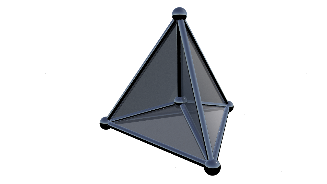
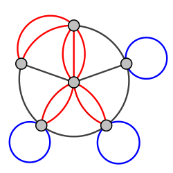
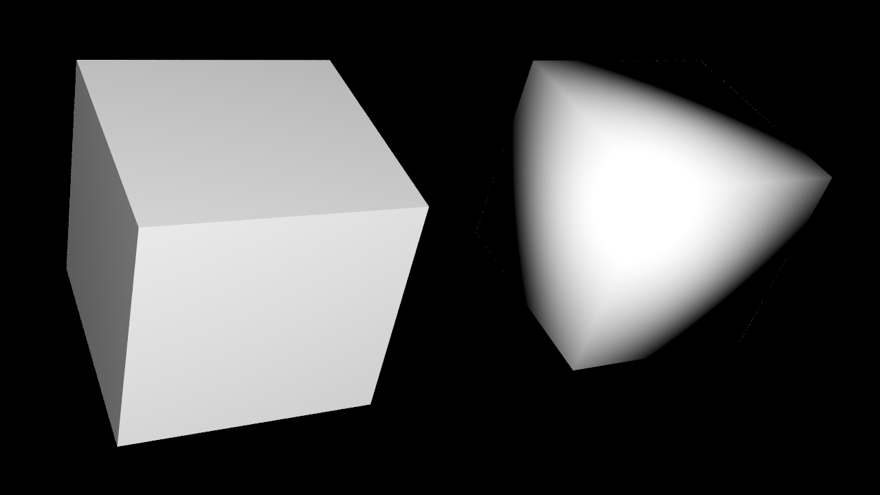
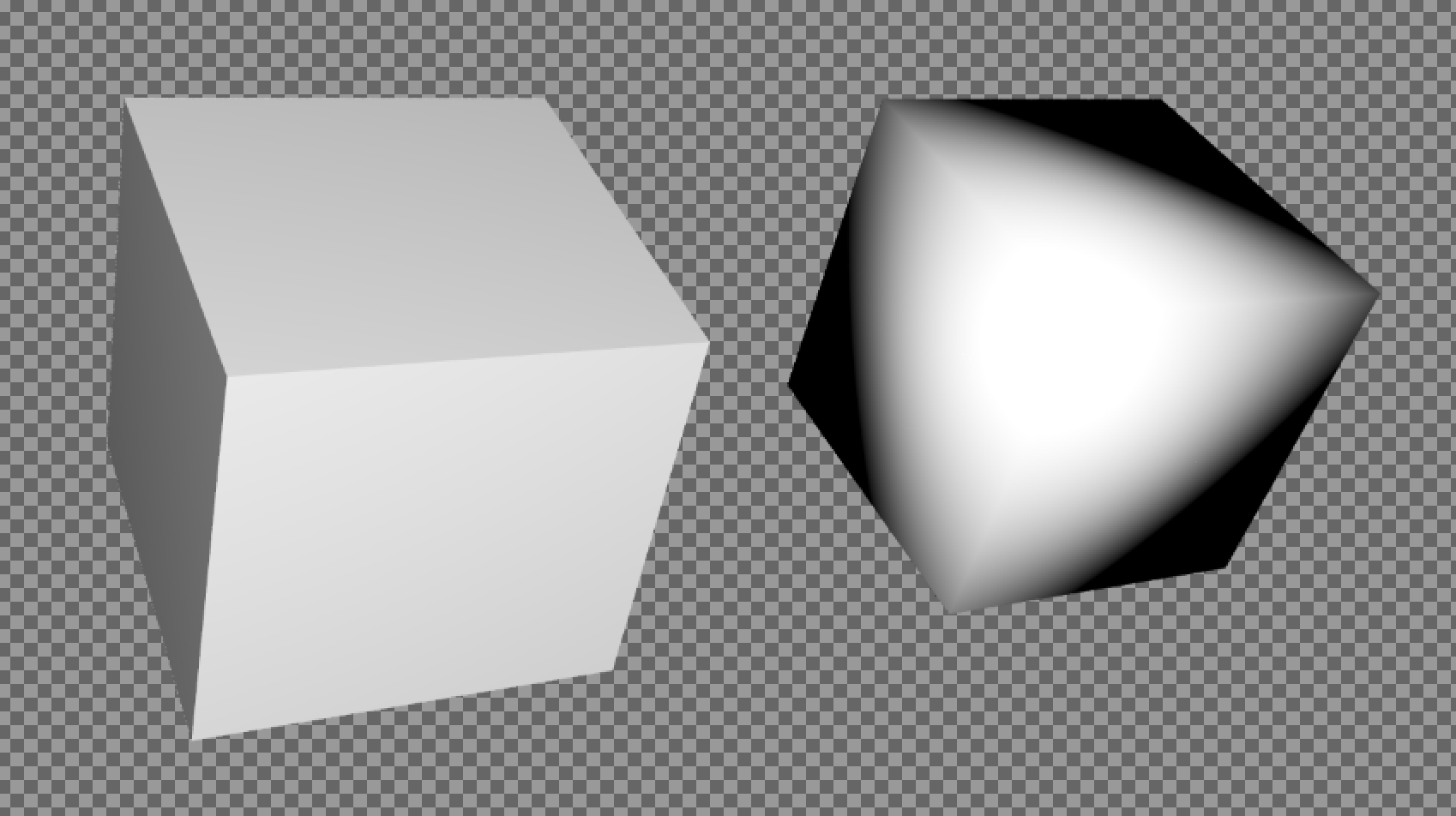
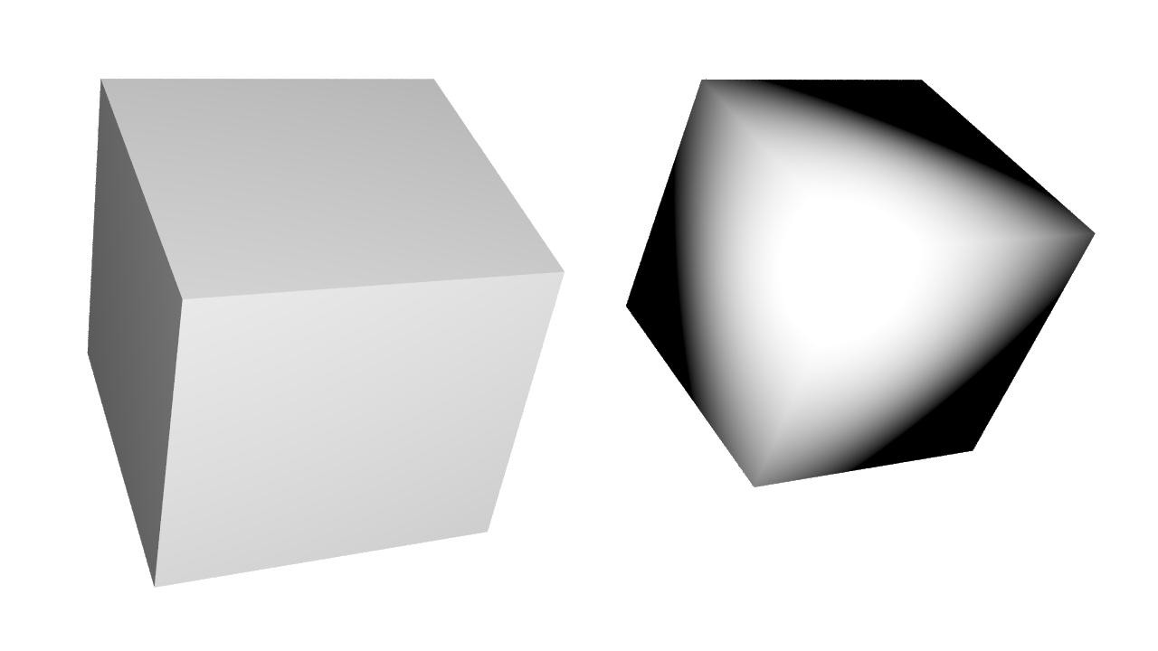
For example we already showed several times a cone over the one-skeleton of a tetrahedron. To create this geometry in Houdini on can use an Attribute Wrangle node and paste into the text field labeled “VEXpression” the following code:

Here you also see how to define custom functions in VEX. For a general introduction to VEX we refer to the documentation. The same task could also be accomplished with a Python node. The necessary Python code looks as follows:

wheel-11

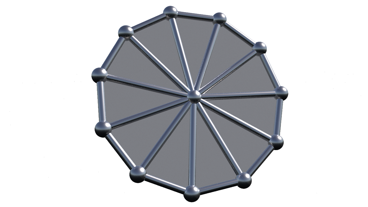
It is also possible to add interactive parameters to nodes. As an example we create a wheel with a variable number of spokes: Create a node of type Attribute Wrangle. Add a parameter of type float named numSpokes with label “number of spokes” to the node (see the documentation for the details how to do this). The needed VEX code is the following:

Posted in Lecture | Comments Off on Creating Geometry From Scratch

Combinatorial Geometry in Houdini

As primitive geometric objects (objects that do not arise as combinations of other objects) Houdini supports also round spheres, cylinders (called tubes in Houdini), volumes and other things. We will focus here on Houdini’s implementation of the combinatorial complexes described in the last two posts.

Both types of complexes that we discussed rely on a finite set $P$ of points. This is the case also in Houdini. Since Houdini wants to visually represent all of its geometry, here every point $i$ comes with a position $\mathbf{p}_i\in \mathbb{R}^3$.

All combinatorics in Houdini is encoded in a finite set of polygons. Polygons come in two flavors, open or closed. In both cases the polygon is described by an arbitrary finite sequence

\[\gamma = (i_1,\ldots,i_n)\]

of points $i_1,\ldots,i_n \in P$. If a polygon is marked as “open”, it will be drawn by connecting in $\mathbb{R}^3$ the positions $\mathbf{p}_{i_k},\mathbf{p}_{i_{k+1}}$ of consecutive points by straight line seqments.

polygon2

If the polygon is marked as “closed”, there will be also a line seqment from $\mathbf{p}_{i_n}$ to $\mathbf{p}_{i_1}$ and the polygon will be rendered as filled in by some surface (which looks more smooth in the render view than in the scene view).

 closed-polygon-2

What is now the relation of Houdini’s setup to the two types of combinatorial complexes that we discussed?

First, based on Houdini’s data we define a one-dimensional simplicial complex $\Sigma$: A two-element subset $\{i,j\}\subset P$ belongs $\Sigma$ if and only if there is a polygon $\gamma = (i_1,\ldots,i_n)$ and an index $k$ such that $(i,j)=(i_k,i_{k+1})$. Here the indices are understood modulo $n$ in case the polygon $\gamma$ is closed.

Next, we make $\Sigma$ into a one-dimensional cell complex (a multigraph) $G$ which has oriented edge starting at $i$ and ending at  $j$ if and only if $\{i,j\}\in \Sigma$.

Finally, we create a two-dimensional cell complex whose faces $\varphi\in F$ correspond one-to-one with the closed polygons: To each closed polygon $\gamma$ we assign the edge cycle in $G$ corresponding to $\gamma$.

So there are no edges in Houdini’s underlying combinatorial data structure, edges are derived quantities here. However, Houdini provides two convenient ways to access the resulting edge graph $\Sigma$: First, there is a node named “Convert Line” that provides a two-vertex open polygon for each edge of $\Sigma$. Second, there are two methods findEdge and globEdges on the Python class hou.geometry that provide access to $\Sigma$.

Besides this, there are of course many interactive tools that work with edges.

Posted in Lecture | Comments Off on Combinatorial Geometry in Houdini

Combinatorial Geometry: Simplicial Complexes

While (for good reasons) we have restricted our treatment of combinatorial cell complexes to the two-dimensional case, the theory of $n$-dimensional simplicial complexes is rather straightforward:

Definition: A simplicial complex is a finite set $P$ together with a set $\mathcal{S}$ of subsets $S\subset P$ with the following properties:

(i) For every $i\in P$ we have $\{i\}\in \mathcal{S}$.

(ii) If $S\in\mathcal{S}$ and $T\subset S,\,T\neq \emptyset$ then $T\in \mathcal{S}$.

An element $S\in\mathcal{S}$ is called a simplex of $\mathcal{S}$ of dimension $k$ if the number of its elements equals $k+1$. The set of all $k$-dimensional simplices in $\mathcal{S}$ is called the $k$-skeleton $\mathcal{S}^k$ of $\mathcal{S}$.

A one-dimensional simplicial complex is the same thing as a graph. The one-dimensional simplices of any simplicial complex are called edges, the two-dimensional simplices are called triangles and the three-dimensional ones are called tetrahedra. The picture below shows a graph with $P=\{1,2,3,4,5,6\}$ and seven edges.

graph

A one-dimensional simplicial complex $\mathcal{S}$ (a graph) can be viewed as a special one-dimensional cell complex $M$ (i.e. a special multigraph). The oriented edges of $M$ is the set of ordered pairs $(i,j)$ with $\{i,j\}\in \mathcal{S}^1$ and the maps $s,d,\rho$ are defined by

\begin{align*}s((i,j))&:=i\\ d((i,j))&:=j \\ \rho((i,j))&:=(j,i).\end{align*}

Similarly, a two-dimensional simplicial complex can be viewed as a special two-dimensional cell complex. The cell-complex below from the last post arises in this way from a two-dimensional simplicial complex with five points, ten edges and six triangles.

tet-cone-simple

We have not really discussed this, but a two-dimensional cell complex describes a unique topological space. The same holds for general simplicial complexes. However, simplicial complexes are much more powerful for the discrete modeling of physical objects for the following reason: The topological space described by a combinatorial simplicial complex comes with a canonical piecewise affine structure. We now elaborate what this means.

Let $\mathcal{S}$ be a simplicial complex with point set $P$. Define then the piecewise affine space $C(\mathcal{S})$ corresponding to $\mathcal{S}$ as the set of all functions $f:P\to \mathbb{R}$ such that  $f(i)\geq 0$ for all $i\in P$,

$$\sum_{i\in P}\, f(i)=1$$

and

$$\big\{ \,i\in P \,\,\,\big|\,\,\, f(i)\neq 0\,\big\} \in \mathcal{S}.$$

For each simplex $S\in \mathcal{S}$ we define an affine space

$$\mathcal{A}_S:= \bigg\{\, g: P\to \mathbb{R} \,\,\,\bigg|\,\,\,\sum_{i\in P} g(i)=1\mbox{   and   }i\notin S \implies g(i)=0 \,\bigg\}$$

The vector space corresponding to the affine space $\mathcal{A}_S$ is

$$V_S:= \bigg\{\, g: P\to \mathbb{R} \,\,\,\bigg|\,\,\,\sum_{p\in P} g(i)=0\mbox{   and   }i\notin S \implies g(i)=0 \,\bigg\}$$

and each $\mathcal{A}_S$ is spanned by the simplex

$$\Sigma_S:=\big\{\, g\in\mathcal{A}_{S} \,\,\,\big|\,\,\,g(i)\geq 0 \mbox{   for all   } i\in P \,\big\}.$$

The whole space  $C(\mathcal{S})$ is the disjoined union of all the interiors (within $\mathcal{A}_S$) of the simplices $\Sigma_S$ for $S\in \mathcal{S}$. If $S\in \mathcal{S}$ and $T\subset S$ then $\mathcal{A}_T$ is an affine subspace of $\mathcal{A}_S$. Similarly, we also have $\Sigma_T \subset \Sigma_S$ in this case.

Each point $i\in P$ corresponds to a particular element $\delta_i\in C(\mathcal{S})$ defined by $\delta_i(j)=1$ for $j=i$ and $\delta_i(j)=0$ otherwise. We have $\mathcal{A}_{\{p\}}=\Sigma_{\{i\}}=\{\delta_i\}$. The main property that makes simplicial complexes useful for physical modeling is the following easy-to-prove

Theorem: Let $\mathcal{S}$ be a simplicial complex with point set $P$ and let  $f: P \to V$ be a map into any vector space $V$. Then there is a unique map

$$\hat{f}:C(\mathcal{S})\to V$$

whose restriction to each simplex $\Sigma_S$ is affine and which extends $f$ in the sense that for all $i\in P$ we have

$$\hat{f}(\delta_i)=f(i).$$

In particular, if we have a two-dimensional simplicial complex and are given a position in $\mathbb{R}^3$ for each of its points, it is clear how to fill in the triangles, for example in order to render them.

Posted in Lecture | Comments Off on Combinatorial Geometry: Simplicial Complexes

Combinatorial Geometry: Cell Complexes

Roughly speaking, Combinatorial complexes play a similar role in the discrete world as differentiable manifolds in the smooth world. They are able to capture the “intrinsic” properties of a geometric object, i.e. those properties that are independent of any embedding into an ambient space.  Combinatorial complexes come in two flavors: cell complexes and simplicial complexes. In this post we deal with the former.

A one-dimensional combinatorial cell complex is the same thing as a finite multigraph. Such a multigraph $M$ is given by

  • a finite set $P$ of “points”.
  • a finite set $\tilde{E}$ of “oriented edges”.
  • maps $s,d: \tilde{E}\to P$ assigning to each oriented edge its “source point” $s(e)$ and its destination point $d(e)$.
  • a map $\rho: \tilde{E}\to \tilde{E}$ that implements “orientation reversal”: We demand that for all $e\in\tilde{e}$ we have $\rho(e)\neq e$ and $\rho\circ \rho(e)=e$. Moreover we assume

\begin{align}s\circ \rho &= d \\ d\circ \rho &= s.\end{align}

Note that what we call “points” usually would be called “vertices”. We use “points” in order to remain consistent with Houdini terminology. A two-element subset $\hat{e}\subset\tilde{E}$ of the form $\{e,\rho(e)\}$ is called an (unoriented) edge of $M$.

A typical multigraph looks like this:

Multi-pseudograph

You see that there can be several edges connecting the same pair of points and there can be oriented edges whose source and destination point coincide. There also could be isolated points that do not belong to any edge.

A two-dimensional combinatorial cell complex is a one-dimensional cell complex $G$ together with a set $F$ of faces, where to each face $\varphi$ there is assigned a corresponding “edge cycle” of $G$. What is an edge cycle?

An edge loop in a one-dimensional cell complex $G$ is a finite sequence $(e_1,\ldots,e_n)$ of oriented edges in $G$ such that for $1\leq j\leq n$ we have

\[d(e_j)=s(e_{j+1})\]

and $d(s_n)=s(e_1)$. An oriented edge cycle in $G$ is an equivalence class of edge loops where two edge loops are considered equivalent if they only differ by a cyclic permutation of the edges. Similarly, we obtain an unoriented edge cycle (or briefly an edge cycle) if we also allow reversing the order of the loop.

$G$ is called the 1-skeleton of the two-dimensional combinatorial cell complex $M$. Here is a visualization of a two-dimensional combinatorial cell complex with five vertices, ten edges and six faces:

tet-cone-simpleNote that different faces can have the same edge cycle. This is for example the case for the sphere below, which is represented as a two-dimensional cell complex with six points, six edges and two faces:

lens-iron

A two-dimensional combinatorial cell complex $M$ can be considered as a description of a certain topological space $\hat{M}$, a so-called two-dimensional cell complex. An $n$-dimensional cell is just the unit ball $B^n\subset \mathbb{R}^n$, considered as a topological space.

  • The points $p\in P$ of a two-dimensional combinatorial cell complex the represent $0$-cells. This cloud $P$ of isolated points is called the $0$-skeleton $\hat{M}_0$ of the cell complex $\hat{M}$.
  • Each edge $e\in E$ corresponds to a copy of the intervall $[-1,1]$ (the unit ball in $\mathbb{R}^1$). The end points of this 1-cell are identified with the end points of $e$ prescribed by the combinatorics. The topological space that results from this gluing is called the $1$-skeleton $\hat{M}_1$ of $\hat{M}$.
  • Corresponding to each face $\varphi\in F$ we have a $2$-cell $c_\varphi$, i.e. a copy of the unit disk $B^2\subset \mathbb{R}^2$. The boundary $\partial c_\varphi$ of each $1$-cell is homeomorphic to the unit circle $S^1$. Up to topological equivalence there is a unique map of $\partial c_\varphi$ to the $1$-skeleton $\hat{M}_1$ that fits the edge cycle of $\varphi$. The space obtained from gluing in this way the boundaries of all $2$-cells to the 1-skeleton $\hat{M}_1$ finally is the 2-dimensional cell complex $\hat{M}$.

See the Wikipedia articles on abstract cell complexes and CW-complexes for further information.

Two-dimensional combinatorial cell complexes are very common in Computer Graphics. In particular, what usually is called a “polygonal surface” is a two-dimensional combinatorial cell complex $M$ together with a map $P\to \mathbb{R}^3$ that gives each point a position in space.

Note however that it is not even clear how to render a face $\varphi$ of such a polygonal surface if the points on the boundary cycle of $\varphi$ are positioned on a plane. The same problem arises for numerical computations in the spirit of finite elements that need to extend quantities given on the boundary of a face to its interior. This is the reason why for many practical applications simplicial complexes are more adapted than cell complexes. We will study these in the next post.

Posted in Lecture | Leave a comment

Scenes with White Background

In a scientific context a very common task is to prepare figures for manuscripts. In most cases the objects in the foreground are the sole focus of attention, and in such cases it is desirable that the figure should blend naturally with the surrounding page. This means that often the goal is to have a white background. Nevertheless, shadows are frequently included in order to give at least a minimal sense of spatial orientation.

Let us illustrate how to achieve this by starting with the scene from the last post. First we turn off Render Light Geometry in the Light tab of the Sky Light. This has no effect in the Scene View but in the Render view the sky turns white (at least if you adjust the Display Options of the Render view as explained in a previous post):

truncated-with-white-sky

Giving the ground a white material probably would not make it completely white. To make the ground white we in fact will use a marvelous material called “Shadow Matte”. An object mad of this material (assuming we use the default settings) will cast shadows on other objects but will be rendered as transparent portions of the image, so when composed onto another image (or a white page) the background will shine through at the places where the object is visible. Most importantly, shadows on the object will be accumulated as opaqueness (of a color that depends on the corresponding light color). Here is the result:

truncated-with-ground-off-render-white-bg

You will notice that the sky light creates a faint shadow that was hardly noticeable against the clay material. This shadow prevents us from perfect blending with the white page, so we turn it off: In the Shadow tab of the Sky Light node we replace the “*” in the Shadow Mask parameter by “ground” (referring to the node we renamed to “ground”). This means that as far as the sky light is concerned only the ground will cast shadows, not the polyhedron:

 truncated-clean-shadow

The shadow will look more appealing if we make the faces partially transparent. So let us delete the White Porcelain material from the Geometry node and inside of it replace both Color nodes by Material nodes. Assign the Iron material in both Material nodes. Place a Material node also below the Facet node and make it represent a Mantra Surface material. In the parameter interface of this Mantra Surface material set the Opacity Scale on the Opacity tab to 0.5. The result is this:

truncated-transparent-white

Very often an appropriate use of transparency can substantially increase the amount of information carried by a picture.

Posted in Lecture | Leave a comment

Simple Ambient Scenes

Visual perception is always slightly irritated when it is confronted with understanding objects that are just floating in empty space, with no clues concerning the surrounding environment. For this reason the slight gradient in Houdinis Scene View is already helpful: The darker color at the top of the window creates the impression of spatial depth. A uniform color would be visually more disconcerting.

So even if we only want to investigate a single object, it is often desirable to place the object in some simple unobtrusive environment and provide the corresponding lighting.

Let us start with the ball-and-stick platonic solid of the last post, only this time with a truncated dodecahedron (called a “Soccer Ball” in the menu).

truncated-no-material

We begin by assigning a more sophisticated material to the whole object. Materials that we want to use are collected in the Material Palette, which is available as a tab on the Network View. In the list of available materials on the left find White Porcelain and drag it to the empty pane on the right. Now we zoom out of the geometry node, which is most conveniently achieved by typing “u” (for “up” in the hierarchy versus “in” to open up a node…). There we select the Geometry node that contains everything else. In its parameter interface select the Material tab. Click on the symbol that looks like a node with a mouse pointer over it. You get a list of all available materials (visible after expanding the “Shop” node). Select White Porcelain and hit the Accept button. Here is the result:

truncated-with-material

Next we add some light. A very convenient setup is provided by the Sky Light node. Place such a node on the top level of the network (next to the Geometry node). You will see two nodes appear, one containing the light that represents the sun and another one for the rest of the sky. All editing is done on the sky node (of type Environment Light), the settings of the sun will follow automatically. The most useful control determines the elevation of the sun (45 degrees by default), i.e. the time of the day. Varying this parameter we will get sky colors that are computed according to some standard physical model.

truncated-with-skylight

We want to see the sky also in the Render View, so we make a checkmark next to “Render Light Geometry”. The rendered image looks like this:

truncated-with-skylight-render

Still our truncated dodecahedron looks like floating in high altitude above a green landscape. So let us add some ground. On the top level of the network create another Geometry node and rename it to “ground”. Dive into it and create a Circle. Set its Orientation to “ZX Plane”, its Center to (0,-1.2,0) and its Scale to 100. Zoom out, add the material Clay to the Material Palette and assign it to the ground node. In the Scene View the change is not very spectacular:

truncated-with-ground

However, in the Render View the ground shields off the light from the lower half of the sky and receives a shadow:

truncated-with-ground-render

Adjusting the camera a bit we see the full shadow:

truncated-with-ground-off-render

Posted in Lecture | Leave a comment

Visualizing Discrete Geometry with Houdini II

Let us now work on the visualization of edges and points. In case you worry that your screen looks slightly different from the pictures we show: For the pictures we already applied the White Porcelain material as explained in the next post (the difference is not large).

Start with a Platonic Solids node providing a dodecahedron and connect below it a Facet node as in the previous post.

dodecahedron

Now feed the dodecahedron into a node of type Wireframe and in the parameter interface of this node set Wire Radius to .04. Connect below Wireframe a node of type Color and choose a color you like. Use a node of type Merge (see the previous post) to display the faces and the edges together. The result will look like the picture below.

dodecahedron-with-edges

Now create a Sphere node, set the sphere radius to 0.1 and connect below it another Color node to makes the sphere red. Feed the result into the left input of a Copy node and connect the right input of this node to the output of Platonic Solids. Copy will translate a copy of the object in its left input to every point of the geometry in its right input.

dodecahedron-with-edges-and-points

This kind of visualization is reminiscent of the ball-and-stick models used in molecular Chemistry. It is quite useful for working with coarse polyhedral geometries. Here is the final network:

ball-and-stick-network

Why did we put a node of type Null below the Platonic Solids node? This is because we then can select all nodes except Platonic Solids and choose “Collapse” from the context menu (right mouse button) of the Network View. This will reduce the visual clutter of more complicated networks. Moreover, we can then save the collapsed as a so-called digital asset. In fact, if you installed the ddg asset library coming with this course, you will have this node available in the tab menu under the name Ball and Stick.

Posted in Lecture | Leave a comment

Rendering and Working with Cameras

Before rendering it is always convenient to create a dedicated camera for this purpose. You do this by choosing New Camera from the yellow menu in the upper right corner of the Scene View. After this, you will see a rectangular region in the Scene View that shows the scene as seen by this camera. If you want to change the perspective of this camera, you can highlight the lock icon on top of the vertical tool bar on the right of the Scene View. If afterwards you unlock the view again you can look around freely without messing up the camera meant for rendering. You can switch the Scene View back to this camera by selecting its name (often something like “cam1”) it the mentioned yellow menu. You can have as many cameras as you like. They will show up as nodes on the top level of the network, next to the Geometry node that you initially created.

Now switch from the Scene View to the Render View. You can do this by selecting the appropriate tab at the top of the scene view window. You will see the scene through the eyes of the camera selected in the ROP Camera menu above the scene view. For example, the scene from the last post looks like this:

cube-facets

Why do we see a black background? In fact, in reality the background is not black but transparent. You can see this if you save the image (using the context menu available on the Render View, right mouse button) in a format like png that supports transparency. If you open the saved image in image software like GIMP you will see the transparency:

cube-facets-gimp

The same image loaded in a web browser will feature the background color  of the current browser page, in our case white:

cube-facets

Obviously it seems desirable to see the rendered image in front of the envisaged background also in the Render View. To this end, click on the vertical rectangle on the right of the Render View to exhibit its tool bar. The uppermost icon in this toolbar gives access to the Display Options of the Render View. This pop up window has a tab called “Background” where you can change the background color from (0,0,0) to (1,1,1). In order for this change to have effect we also have to highlight the icon on the Scene View toolbar that is labelled “Toggle Transparency”.

Note that if you save your image in a format like JPEG that does not support transparency, you will always see a black background on the image. The background of the Render View only affects the preview. We strongly recommend saving your images with transparency, also if they are meant for videos. In this way you maintain full flexibility concerning the background that you finally will use.

Posted in Lecture | Leave a comment

Visualizing Discrete Geometry with Houdini I

This post is also meant as a first introduction to using Houdini.

In most applications discrete curves and surfaces are used as approximate descriptions of smooth objects. This situation is close in spirit to Numerical Analysis where the discrete objects would be considered as approximations by “finite elements” of some smooth geometry.

In Discrete Geometry the polyhedral surfaces themselves are the prime focus of study. The emphasis here is often on questions of combinatorics and many arguments have the flavor of Elementary Geometry.

Also in Discrete Differential Geometry the discrete objects are studied in their own right. However, the goal is to develop a theory that corresponds as closely as possible to the theory of smooth curves and surfaces. Questions of convergence in the continuum limit are still marginally interesting. They are however not as central as they would be in in Numerical Analysis. InDiscrete Differential Geometry the question remains interesting how the theory performs if the discrete objects have only very few vertices.

Both in the context of Discrete Geometry and the context of Discrete Differential Geometry the wish sometimes arises to render discrete curves and surfaces in a way that gives more prominence to individual vertices, edges and faces:

  • In classical geometry drawings it is customary to draw distinguished points as small circles. The analog of this in a computer-aided three-dimensional context is to display points as small spheres.
  • The orientation of straight lines in three dimensions becomes much more clearly evident if the line is drawn as a thin cylindrical tube with appropriate lighting.
  • The spatial orientation of planar faces is easier to discriminate if appropriate lighting is applied.

When Houdini first starts up there are three main windows (aside from the menu [top] and status [bottom] bars). On the left the “Scene View,” while on the right we have the parameter editor (top) and the “Network View” which will be our main interaction window for creating node networks.

Let us start with the facets. Start up Houdini and create a Geometry node. To this end make sure the focus is in the node editor window (bottom right) and hit the Tab key. A menu with a list of all available node typed will pop up. Start typing “g” and you will see a list of all node types whose name starts with “g”. If you go on typing to complete the name “geometry”, already after one more keystroke the choice will narrow down to a unique one. Now you can either hit the Enter key or click on the only remaining menu item labeled “Geometry”. A rectangular outline will appear in the Network View that allows you to place the node at a position of your choice. As soon as it is placed the parameter editor window above will show the parameters associated with the currently highlighted node in the network editor.

Dive into the newly created geometry node by double-clicking on it. Inside you will find a node providing the standard test geometry. Select it by clicking on it and delete it by using the Delete key. Instead of the standard geometry we will attach a geometry of our choosing. To do so, create a node of  type Platonic Solids. Once again do this by hitting Tab and starting to type “Plato…” and place the node. In the upper right panel of the Houdini window (the parameter window) you will see the parameters associated with the Platonic solid node. Use the dropdown menu labeled “Solid Type” to select “Cube.” You will see something like the cube on the right in the picture below. If you make sure that the camera symbol visible on the left vertical toolbar (left of the scene view window) is selected, you can rotate the whole scene (actually you rotate the camera) using the left mouse button and translate it using the middle mouse button. You can toggle the grid on or off by clicking on the uppermost symbol on the right (of the scene view) vertical toolbar.

cube-facets-view

The lighting of this cube seems strange. The reason is that by default Houdini treats all discrete surfaces as approximations to smooth ones, so it is only natural to treat the cube as a coarse approximation to something like a round sphere. This becomes more apparent if we show the normals: From the yellow menu in the upper right of the Scene View labeled “persp1” choose “Display” and make a checkmark next to “Normals” (alternatively find the “display normals” icon button on the right vertical tool bar in the scene view window).

cube-facets-normals

Normals are interpolated across the surface for shading purposes. Here we see that the cube has only a single normal at each vertex. On the other hand, the cube on the left shows three different normals at each vertex, one for each adjacent face. This is what we want. So we have to find a way to tell Houdini that we really mean a surface with planar faces which make sharp angles.

We can achieve this by placing a node of type Facet below the Platonic Solids node. Same as before: be sure focus is in the network editor window, hit TAB and start typing “Fac…” After placing the box connect the output of the node of type Platonic Solids to the input of the node of type Facet: Click on either port with the left mouse button, release the button, move over to the other port and click again.

In the upper right corner the parameter interface of the Facet node is accessible. There check Cusp Polygons, which means that all edges between faces that make an angle bigger that the Cusp Angle displayed right below will be treated as sharp angles. 20 degrees (the default number already there) would be small enough for the cube, but we might as well type in zero here. By this we indicate that all edges between faces are to be treated as sharp edges. So far you don’t see any change in the Scene view. This is because the “Display/Render” button is highlighted still in the “platonic” box (it is the rightmost blue rectangle in that block). Now click on the rightmost rectangle on the Facet node in order to make it the current Display node. Now we see the cube with the shading that we intend.

In order to make the pictures shown above we placed the original cube side by side by its faceted version. For this we used two nodes of type Transform to rotate the original cube and to translate one version of it. These transformations can be typed into the parameter windows (useful when you want precise values), or they can be chosen interactively. For the latter, select one of the transforms. Then in the Scene View select the “Show Handle” button. Play with the handle that comes up. It will allow for constrained and free hand motions. In the end we used a node of type Merge in order to combine the two resulting cubes in one single object:

cube-network

Notice that you will see different things in the Scene view depending on which node has the blue box checked. Also play with the parameters in each node.

Posted in Lecture | Leave a comment

Using Houdini on MacBooks

On Notebooks that are not totally ancient and run Windows or Linux, Houdini works fine. On those Macs that feature a non-Intel graphics chip, Houdini runs excellently. The only problem are Macs with Intel graphics. Here (probably due to the lack of OpenGL 3.0 drivers supplied by Apple) the main interactive viewport switches to software rendering. What follows is a setup that makes it possible to nevertheless do useful work in this situation:

  • Delete the panels labeled “Scene View” and “Animation Editor”.
  • From the “Window” menu choose “New Floating Panel”.
  • Make the resulting window quite small.
  • Right-click in the upper left corner of this window on the tab labeled “/obj” and choose “Scene View”.
  • In the upper right corner of the appearing viewport click on “persp1” and choose “Shading -> Wireframe Ghost”.

Now you can create some geometry and hit the render button in the large “Render View” that you see. From now on you should be able to work smoothly in the small Scene View while after a very short time you will see a nicely rendered image appear in the Render View.

römer

This feels like a setup that one get used to. For us mathematicians the main work will happen anyway in the network editor and the control panels of the nodes. This means that now I am fully determined to base my class that starts in April on Houdini.

Posted in Lecture | Leave a comment